Randomness of Shapes and Statistical Inference on Shapes via the Smooth Euler Characteristic Transform

Figures & data

Fig. 1 Left: Molars from two suborders of the primates: Haplorhini and Strepsirrhini. The Haplorhini suborder has genera Tarsius (yellow) and Saimiri (grey). The Strepsirrhini suborder has genera Microcebus (blue) and Mirza (green). Right: Relationship between the four primate genera. Tarsier molars exhibit additional high cusps (highlighted in red). A similar figure was published in Wang et al. (2021).

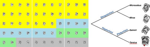
Fig. 2 Consider the two-dimensional shape $K\in {\mathcal{S}}_2$ in the left panel. For each pair of ν and t, the equation $x·\nu =t-R$ represents a straight line (or a hyperplane in a high-dimensional space). The subset $K_t^{\nu }$ denotes the region below this line. Let ${\varphi }_{\nu }(x)=x·\nu +R$, then $K_t^{\nu }=\{x\in K|{\varphi }_{\nu }(x)\le t\}$. The right panel presents the function $(\nu ,t)\mapsto \text{SECT}(K)(\nu ,t)$, where $\nu \in {\mathbb{S}}^1$ is identified by $\theta \in [0,2\pi ]$ through $\nu =(\hspace{0.17em}\mathrm{\text{cos}}\hspace{0.17em}\theta ,\hspace{0.17em}\mathrm{\text{sin}}\hspace{0.17em}\theta )$. Procedures for generating the shape K and the right panel are given in Appendix D.1.

Table 1 Rejection rates (from 1000 experiments) for different indices ε (significance $\alpha =0.05$).

Indices ε	0.00	0.01	0.02	0.03	0.04	0.05	0.06	0.08	0.10
Algorithm 1	0.118	0.161	0.315	0.519	0.785	0.910	0.975	0.990	1.000
Algorithm 2	0.046	0.054	0.162	0.343	0.612	0.789	0.931	0.994	1.000
Algorithm 3	0.050	0.050	0.111	0.185	0.335	0.535	0.739	0.983	0.999
FP	0.136	0.153	0.308	0.539	0.810	0.924	0.986	0.997	1.000
TRP-WTPS	0.075	0.091	0.261	0.515	0.790	0.929	0.980	0.997	1.000

NOTE: Appendix J provides a comparison of Algorithms 1, 2, and 3 to other existing fdANOVA methods.

Table 2 P-values of Algorithms 1, 2, and 4 for the dataset of mandibular molars.

	Algorithm 1	Algorithm 2	Algorithm 4
Tarsius vs. Microcebus	$<{10}^{-3}$	$<{10}^{-3}$	$<{10}^{-3}$
Tarsius vs. Mirza	$<{10}^{-3}$	$<{10}^{-3}$	0.001
Tarsius vs. Saimiri	$<{10}^{-3}$	$<{10}^{-3}$	$<{10}^{-3}$
Microcebus vs. Mirza	$<{10}^{-3}$	0.009	0.004
Microcebus vs. Saimiri	$<{10}^{-3}$	$<{10}^{-3}$	$<{10}^{-3}$
Mirza vs. Saimiri	$<{10}^{-3}$	$<{10}^{-3}$	$<{10}^{-3}$
Tarsius vs. Tarsius	0.196 (0.220)	0.496 (0.294)	0.527 (0.273)
Overall runtimes (in hours)	$\approx 3$	$\approx 3$	$\approx 20$

NOTE: In the last row, we present the overall runtime for conducting all hypothesis testing tasks using each algorithm.

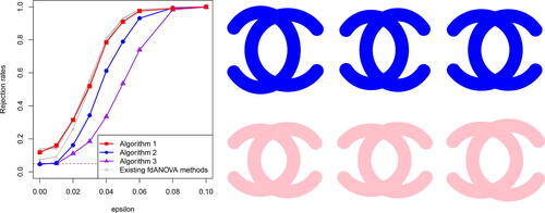
Fig. 3 (Left panel) The relationship between ε and the rejection rates computed via Algorithms 1, 2, 3 (see Table 1), and 12 existing fdANOVA methods (see Table J.1 in Appendix J for details on the existing fdANOVA methods). The (red) dashed line presents the significance level $\alpha =0.05$. (Right panel) The shapes in the first row are from ${\mathbb{P}}^{(0)}$, and the shapes in the second row are from ${\mathbb{P}}^{(0.08)}$.

Wang, B., Sudijono, T., Kirveslahti, H., Gao, T., Boyer, D. M., Mukherjee, S., and Crawford, L. (2021), “A Statistical Pipeline for Identifying Physical Features that Differentiate Classes of 3D Shapes,” The Annals of Applied Statistics, 15, 638–661. DOI: 10.1214/20-AOAS1430.

 Web of Science ®Google Scholar

Data Availability Statement

The source code for implementing the simulation studies and applications is publicly available online at https://github.com/JinyuWang123/TDA.git.