Figures & data
Figure 1. Gaussian denoising: Typical difference between TV (piecewise constant) and TGV reconstructions (piecewise affine).
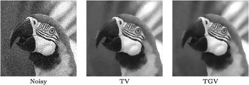
Figure 2. Suitability of the functional as an upper level objective. Evaluation of
where u solves the TGV denoising problem (1.1) (T = Id), for a variety of scalar parameters
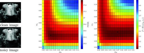
Figure 3. Test images, resolution
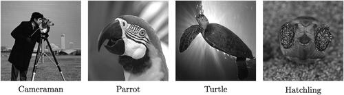
Figure 4. Upper level objective values vs projected gradient iterations for the problem () (right) of (scalar α0, spatial α1).
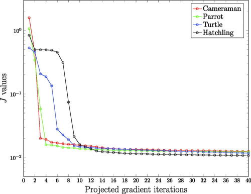
Figure 5. First row: noisy images. Second row: bilevel TV. Third row: Best scalar TGV (SSIM). Fourth row: bilevel TGV.
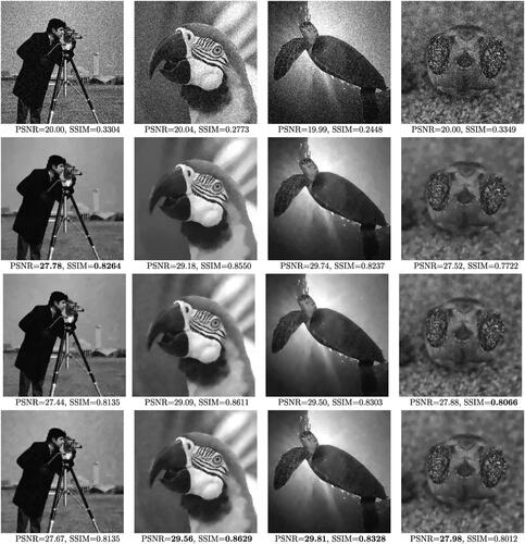
Figure 6. Details of the reconstructions shown in .
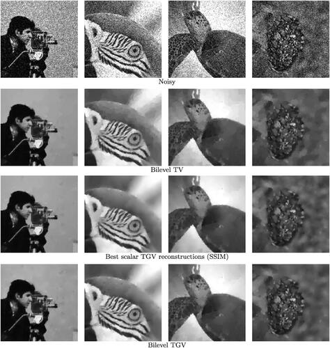
Figure 7. First row: the computed regularization functions α for bilevel TV. Second row: the computed regularization functions α1 for bilevel TGV.
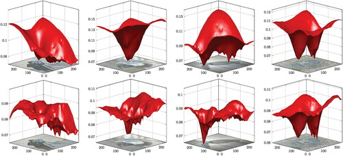
Table 1. PSNR and SSIM comparisons for the images of .
Figure 8. Experiments with optimizing over a spatially varying α0. Top row: the automatically computed scalar parameters α0, that correspond to the images of the last row of . Middle row: the automatically computed spatially varying parameters α0, where α1 has been kept fixed (last row of ). The weight α0 is adapted to piecewise constant parts having there large values and hence promoting TV like behavior, see for instance the parrot image at the last row. On the contrary α0 has low values in piecewise smooth parts promoting a TGV like behavior reducing the staircasing.
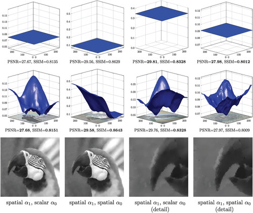
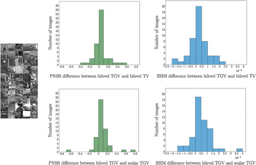
Figure 9. Histograms of the PSNR and SSIM differences between the bilevel spatial TGV and bilevel spatial TV (top) and between the bilevel spatial TGV and bilevel scalar TGV (bottom), for reconstructions of noisy versions of the 50 images on the left. In all bilevel algorithms the ground truth-free statistics-based upper level objective was used.