Figures & data
Figure 1. Sample experimental item for the production experiment: briefing, strong evidence, with colleague interlocutor, discussing suspect Emily Brown.
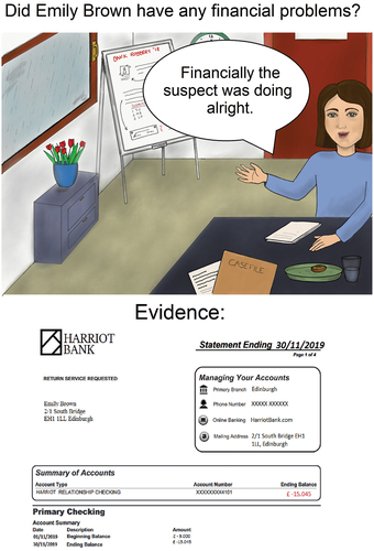
Figure 2. Sample experimental item for the production experiment: Interrogation, weak evidence, with interlocutor suspect Emily Brown.
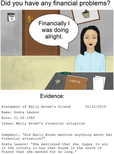
Figure 3. Control item/ attention check briefing in the production experiment.
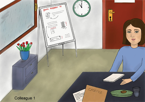
Table 1. Raw counts for each formulation of the production experiment ordered from least frequent to most frequent.
Table 2. Mean evidentiality ratings by formulation and scenario for the production experiment.
Table 3. Population-level estimates of the categorical regression model with interaction in log-odds with the standard errors and 95% credible intervals. In the table the by-expression intercepts are listed first, then the estimates for the evidentiality effect followed by the estimates for the scenario effect and interaction coefficients. Slope coefficients whose 95% credible intervals do not include zero and are therefore treated as reliable effects are highlighted in bold. The effect scenario is the change in log-odds for the briefing (−1 interrogation, 1 briefing). R is a convergence diagnostic whichˆ compares the larger than 1 suggest that the chains have not mixed well.between- and within-chain estimates. Values.
Figure 4. Predictions for the production data. The figure contrasts the two scenarios for each formulation. Log-odds were back-transformed to probabilities (y-axis). The x-axis is the standardized evidentiality measure: 0 stands for an evidentiality of 74.55. An increase of one standard deviation on the standardized scale means an increase of 25 on the original scale. The lines represent the means of the fixed effects, the faded area depicts the 95% credible interval and the darker area the 80% credible interval of the fixed effects.
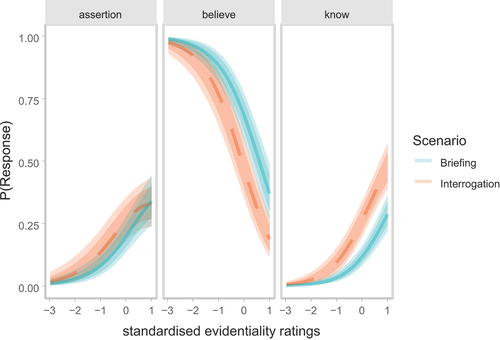
Figure 5. Predictions for the production data. The figure contrasts the three production choices with each other in the two respective scenarios. Log-odds were back-transformed to probabilities (y-axis). The x-axis is the standardized evidentiality measure: 0 stands for an evidentiality of 74.55. An increase of one standard deviation on the standardized scale means an increase of 25 on the original scale. The lines represents the means of the fixed effects, the faded area depicts the 95% credible interval and the darker area the 80% credible interval of the fixed effects.
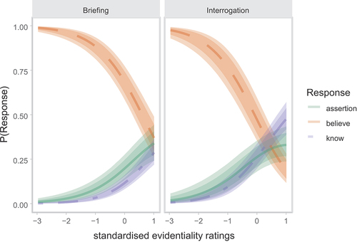
Figure 6. The density plot shows the difference in probability of selecting one of the formulations in the interrogation relative to the briefing for low (green), average (pink) and high evidentiality ratings (blue).
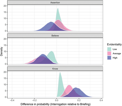
Figure 7. Sample experimental item for the comprehension experiment: briefing, know formulation, with colleagues discussing suspect Emily Brown.

Table 4. Sum coding for the predictor formulation.
Table 5. Mean speaker confidence ratings by formulation.
Figure 8. By-expression speaker confidence ratings for each scenario (briefing in blue, interrogation in red). The figure shows the median of assigned quantities (line) and the upper quartile and lower quartile (box). Whiskers extend to the smallest/largest value within 1.5 times the interquartile range. Dots represent extreme values.
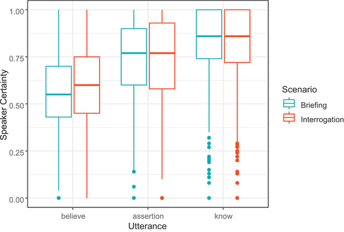
Figure 9. Predictions for the comprehension data. Log-odds were back-transformed to speaker certainty (y-axis). This figure shows the assigned speaker certainties by formulation and scenario (briefing in blue, interrogation in red) with error bars representing the 95% credible intervals.
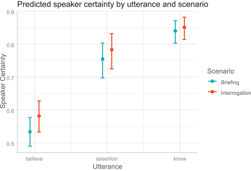
Table 6. Population-level estimates of the Bayesian beta regression model on the log-odds scale with 95% credible intervals. The intercept is the grand mean and translates to 0.74 on the original scale. The categorical predictor formulation was sum-coded, see (4). The coefficient for believe: (−0.83) is the difference between intercept and believe, the coefficient for the bare assertion (0.16) is the difference between intercept and the bare assertion. The difference between the intercept and know can be calculated based on the coding for know, i.e., believe/bare assertion = −1: −0.83 * (−1) + 0.16 * (−1) = 0.67. The effect scenario is the change in log-odds for the briefing (−1 interrogation, 1 briefing). Slope coefficients whose 95% credible intervals do not include zero and are therefore treated as reliable effects are highlighted in bold.
Figure 10. The histogram shows the differences in the assessment of speaker confidence in the interrogation relative to the briefing for believe (Orange), bare assertion (green) and know (violet).
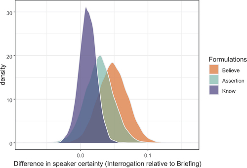
Table A1. Population-level estimates of the categorical regression model in log-odds with the standard errors and 95% credible intervals. In the table the by-expression intercepts are listed first, then the estimates for the evidentiality effect followed by the estimates for the scenario effect. The effect scenario is the change in log-odds for the briefing (−1 interrogation, 1 briefing). R is a convergenceˆ diagnostic which compares the between- and within-chain estimates. Values larger than 1 suggest that the chains have not mixed well.
Table A2. Population-level estimates of the Bayesian beta regression model on the log-odds scale with 95% credible intervals. The categorical predictor formulation was sum-coded. The effect scenario is the change in log-odds for the briefing (−1 interrogation, 1 briefing).
Table B1. Population-level estimates of the categorical regression model in log-odds with the standard errors and 95% credible intervals. In the table the by-expression intercepts are listed first, then the estimates for the evidentiality effect followed by the estimates for the scenario effect. The effect scenario is the change in log-odds for the briefing (−1 interrogation, 1 briefing). R is a convergenceˆ diagnostic that compares the between- and within-chain estimates. Values larger than 1 suggest that the chains have not mixed well.
Table B2. Population-level estimates of the categorical regression model in log-odds with the standard errors and 95% credible intervals. In the table the by-expression intercepts are listed first, then the estimates for the evidentiality effect followed by the estimates for the scenario effect. The effect scenario is the change in log-odds for the briefing (−1 interrogation, 1 briefing). Slope coefficients whose 95% confidence intervals do not include zero and are therefore treated as reliable effects are highlighted in bold. R is a convergence diagnostic which compares the between- and within-chainˆ estimates. Values larger than 1 suggest that the chains have not mixed well.
Table B3. Population-level estimates of the Bayesian beta regression model on the log-odds scale with 95% credible intervals. The categorical predictor formulation was sum-coded, see (4).
Table B4. Population-level estimates of the Bayesian beta regression model on the log-odds scale with 95% credible intervals. The intercept is the grand mean and translates to 0.74 on the original scale. The categorical predictor formulation was sum-coded, see (4). The coefficient for Utterance I (−0.82) is the difference between intercept and believe, the coefficient for Utterance II (0.16) is the difference between intercept and the bare assertion. The difference between the intercept and know can be calculated based on the coding for know, i.e., UtteranceI/UtteranceII = −1: −0.82 * (−1) + 0.16 * (−1) = 0.66. The effect scenario is the change in log-odds for the briefing (−1 interrogation, 1 briefing).
Figure C1. Experimental item: Briefing (suspect Emily Brown, weak evidence).
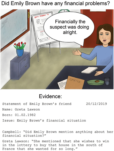
Figure C2. Experimental item: Briefing (suspect Emily Brown, strong evidence).

Figure C3. Experimental item: Interrogation (suspect Emily Brown, weak evidence).
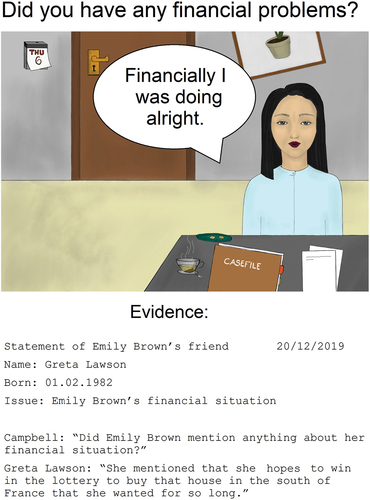
Figure C4. Experimental item: Interrogation (suspect Emily Brown, strong evidence).
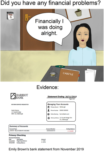
Figure D1. Experimental item: Briefing (suspect Emily Brown/“know”).
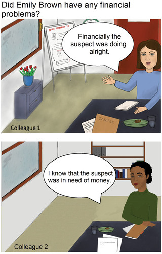
Figure D2. Experimental item: Interrogation (suspect Emily Brown/“believe”).
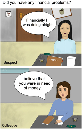
Figure D3. Experimental item: Interrogation (suspect Johanna Smith/“know”).
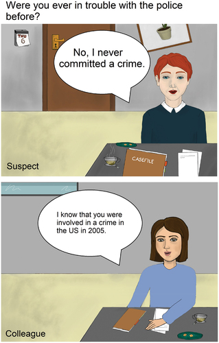
Figure D4. Control item/attention check: Briefing.
Figure D5. Control item/attention check: Interrogation.