Taxonomic revision of Spiniferites elongatus (the resting stage of Gonyaulax elongata) based on morphological and molecular analyses

Figures & data

Table 1. Results from the morphometric analyses of Spiniferites elongatus sensu lato cysts retrieved from surface sediments and sediment trap sequences.

	Area	Production window	Cyst height (µm)	Cyst width (µm)	Antapical process length (µm)	Antapical crest height (µm)
1	Western Hudson Bay	November–December 2005	47	27	9	N/A
2			47	31	12	4
3			56	29	13	N/A
4			49	29	8	N/A
5			48	31	9	N/A
6	Eastern Hudson Bay	November–December 2005	57	29	15	N/A
7			52	26	5	3
8			46	31	8	2
9			55	31	7	4
10			54	32	14	3
11			60	35	8	N/A
12			52	31	18	3
13			54	28	15	4
14			53	33	16	3
15			47	33	5	N/A
16		July 2006	54	33	9	5
17			49	33	14	4
18			58	32	15	7
19			50	34	14	9
20			50	28	22	4
21	Hudson Bay	Surface sediment	61	36	10	N/A
22			49	36	15	3
23			49	31	N/A	N/A
24			52	34	10	4
25			51	38	14	7
26			51	26	11	8
27			58	35	12	5
28			61	35	20	6
29			62	35	16	6
30			56	34	17	3
31			52	32	12	7
32			54	38	16	11
33			51	32	9	6
34			48	33	17	9
35	New England	Surface sediment	59	36	13	8
36			49	25	15	3
37			47	33	9	5
38	Newfoundland	Surface sediment	53	31	10	6
39			54	36	12	4
40			42	27	12	3
41			53	32	15	2
42			57	32	13	6
43			55	35	14	4
44	Omura Bay	Surface sediment	47	23	9	N/A
45			56	30	12	3
46	Alaskan coast	Surface sediment	42	26	10	6
47	Santa Barbara Basin	Surface sediment	46	26	11	2
48	North Bering Sea	Surface sediment	48	32	12	6
49			48	27	12	4
50			56	25	14	8
51			46	27	10	8
52			52	34	11	7
53			51	33	17	12
54			50	33	12	8
55	Chukchi Sea	Surface sediment	53	35	18	10
56			53	38	10	6
57			64	31	15	10
58			51	41	18	8
59			60	37	10	N/A
60			58	37	15	8
61			61	36	21	3
62			63	35	20	6
63			49	30	14	8
64			50	32	17	6
65			60	39	17	5
66			52	31	16	6

Table 2. Location and local surface water conditions for the Beaufort Sea surface sediment samples from which cysts of Spiniferites elongatus sensu lato were isolated.

Station number	Latitude (N)	Longitude (W)	Depth (m)	Temperature^a (°C)	Salinity^a	Cyst^b
ARA05C07	70°27.540	135°46,962	56	6.69	29.40	1, 2, 5, 6, 7, 9
ARA05C05	70°23.766	135°18,816	60	7.22	28.82	3, 4, 8

^a Surface water condition.

^b Numbers correspond to the specimens characterised genetically and illustrated in Plate 1.

Figure 1. Scatter diagram showing cyst width against cyst length for measured elongate Spiniferites cysts. A, Data for all individual measurements from surface sediments. Also shown are the cyst width and length of the holotype of Spiniferites elongatus (black dot) and the topotype extremes (dashed arrow) (Reid 1974), and the average (black Greek cross) and range (black thickened axes) of the cysts measured by Ellegaard et al. (2003), as well as the cyst width and length of the holotype of Spiniferites ellipsoideus (black square) and its type assemblage (grey shaded area) (Matsuoka 1983). B, Average values for each regional surface sediment assemblage, with the standard deviation indicated. Also shown are the values from Harland and Sharp (1986) for specimens recovered from the Firth of Forth (UK), and the Norwegian and Barents seas. C, Individual measurements for the specimens recovered from sediment traps in eastern (EHB) and western (WHB) Hudson Bay.

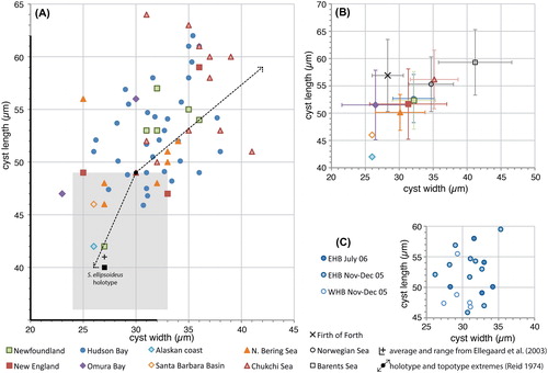
Figure 2. Scatter diagram showing antapical process length against cyst length for measured elongate Spiniferites cysts. A, Data for all individual measurements from surface sediments. The holotype is shown for reference (black dot). B, Average values for each regional surface sediment assemblage, with the standard deviation indicated. Also shown are the values from Harland and Sharp (1986) for specimens recovered from the Firth of Forth (UK), and the Norwegian and Barents seas. Note that the ‘antapical membrane length’ given by these authors (Harland and Sharp 1986, their table 1) is considered to correspond the antapical process length as measured here. C, Individual measurements for the specimens recovered from sediment traps in eastern (EHB) and western (WHB) Hudson Bay.

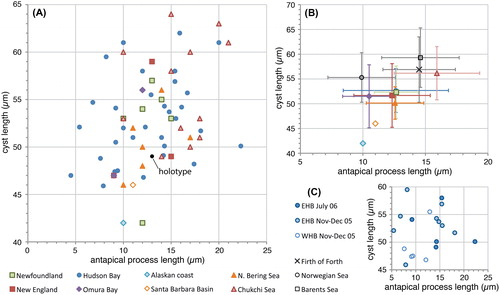
Figure 3. Scatter diagram showing antapical process length against antapical crest height for measured elongate Spiniferites cysts. A, Data for all individual measurements from surface sediments. B, Average values for each regional surface sediment assemblage, with the standard deviation indicated. C, Individual measurements for the specimens recovered from sediment traps in eastern (EHB) and western (WHB) Hudson Bay.

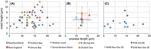
Figure 4. Scatter diagram showing antapical process length against elongateness (i.e. the ratio between cyst length and cyst width) for measured elongate Spiniferites cysts. The holotype is shown for reference (black dot). A, Data for all individual measurements from surface sediments. B, Average values for each regional surface sediment assemblage, with the standard deviation indicated. Also shown are the values from Harland and Sharp (1986) for specimens recovered from the Firth of Forth (UK), and the Norwegian and Barents seas. C, Individual measurements for the specimens recovered from sediment traps in eastern (EHB) and western (WHB) Hudson Bay.

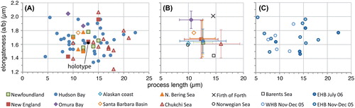
Figure 5. Scatter diagram showing antapical crest height against elongateness (i.e. the ratio between cyst length and cyst width) for measured elongate Spiniferites cysts. A, Data for all individual measurements from surface sediments. B, Average values for each regional surface sediment assemblage, with the standard deviation indicated. C, Individual measurements for the specimens recovered from sediment traps in eastern (EHB) and western (WHB) Hudson Bay.

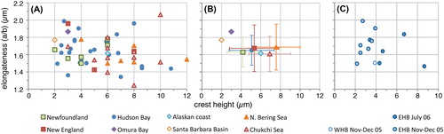
Figure 6. Frequency distribution diagram (A–C: 2 μm bins; D: 1 μm bins) for measured elongate Spiniferites cysts, for the total dataset (blue), cysts from Hudson Bay (red) and cysts from the Chukchi and Bering Sea (green). A) Cyst length; B) Cyst width; C) Antapical process length; D) Antapical crest height.

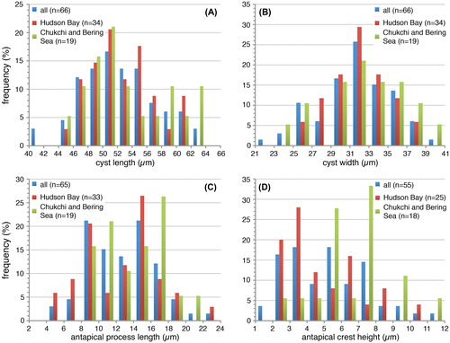
Plate 1. Bright-field photomicrographs of the Spiniferites elongatus sensu lato cysts isolated from the Beaufort Sea that were used in the genetic analyses. The National Center for Biotechnology Information (NCBI) GenBank accession numbers associated to the specimens are KU358942 (cyst 1), KU358943 (cyst 2), KU358944 (cyst 3), KU358945 (cyst 4), KU358946 (cyst 5), KU358947 (cyst 6), KU358948 (cyst 7), KU358949 (cyst 8), and KU358950 (cyst 9). Scale bars = 10 μm.

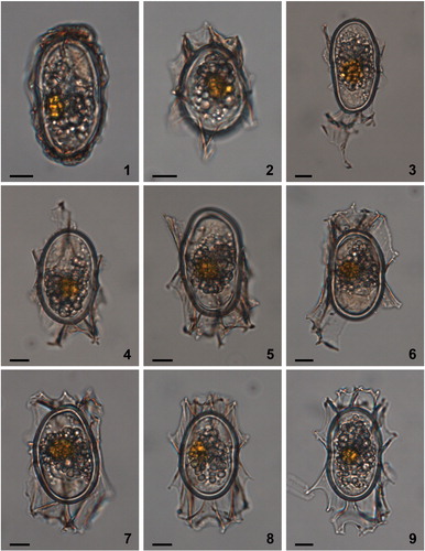
Plate 2. Bright-field photomicrographs of Spiniferites elongatus from off Newfoundland (1–2, 3, 4–5, 6–7) and the Alaskan Coast (8–9). The lines in figure 1 indicate how cyst morphometrics were measured. a = cyst length, b = cyst width, c = antapical process length, d = antapical membrane height. Scale bars = 10 μm.

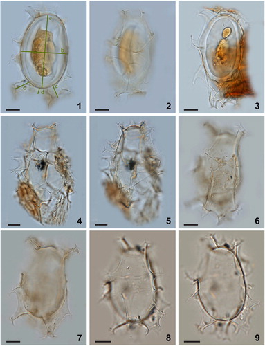
Plate 3. Bright-field photomicrographs of Spiniferites elongatus from Chukchi Sea. 1–3. Dorsal, optical section, and ventral view of a specimen with a high membrane between the two dorsal antapical processes. 4–5. Specimen illustrating the unequal development of the dorsal antapical processes. 6–9. Further illustration of the morphological variability of specimens in a single assemblage. Scale bars = 10 μm.

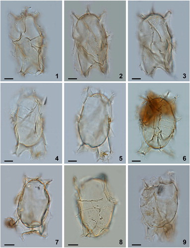
Plate 4. Bright-field photomicrographs of Spiniferites elongatus from (1–6) Hudson Bay surface sediments, (7) eastern Hudson Bay sediment trap deposits collected over July 2006, and (8, 9) western Hudson Bay sediment trap deposits collected from November to December 2005. Note the marked antapical suturocavation in the specimen in figure 7, and the differences in morphology between cysts produced over the same growing season (8 and 9). Figures 1 and 9 are examples of specimens that can be identified as Spiniferites elongatus – Beaufort morphotype. Scale bars = 10 μm.

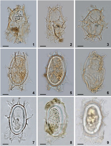
Plate 5. Bright-field photomicrographs of Spiniferites elongatus sensu lato from New England (1, 2, 3), Omura Bay, Japan (4, 5), and the Bering Sea (6–9). While the specimens shown in figures 7–9 are good examples of Spiniferites elongatus – Beaufort morphotype, the specimens shown in figures 4–6 illustrate morphologies somewhat intermediate between typical Spiniferites elongatus and the Beaufort morphotype. Scale bars = 10 μm.

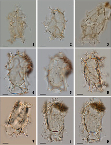
Figure 7. Maximum likelihood (ML) phylogenetic tree based on 799 aligned nucleotides of the nuclear large subunit ribosomal RNA (LSU rDNA) using the TIM3 + G model with Heterocapsa triquetra (Ehrenberg 1840) Stein 1883 and Prorocentrum micans as outgroup taxa. Alignment length includes gaps. The numbers at the nodes of the branches indicate the ML bootstrap (left) and Bayesian posterior probability (right) values; only values ≥50% or 0.5 are shown. Genbank accession numbers are provided.

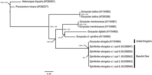
Plate 6. 1–6. Dual interference photomicrographs (1–4) and scanning electron micrographs (5, 6) of Spiniferites elongatus – Norwegian morphotype, from late Pleistocene (Marine Isotope Stage 5e) sediments from the Vøring Plateau, Norwegian Sea. 7–9. Newly produced photomicrographs of the Miocene specimen from Japan that had been designated the holotype of Spiniferites ellipsoideus, herein considered a junior synonym of Spiniferites elongatus. Figures 7–9 courtesy of Kazumi Matsuoka, with kind permission. Scale bars = 10 µm.

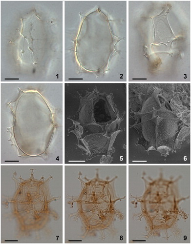
Plate 7. 1–4. Scanning electron micrographs of apical views of four different specimens of Spiniferites elongatus from the Barents Sea with significant variation in the elevation of sutural crests, all showing consistently four apical plates (1′–4′). Note a faint suture between 1′ and 4′. ‘a’ indicates reflection of ventral pore; ‘b’ indicates reflection of apical pore. as = anterior sulcal plate. Scale bars = 10 µm.

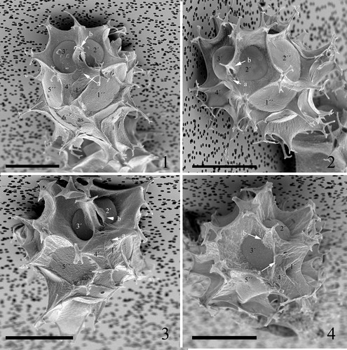
Plate 8. 1–4. Scanning electron micrographs of ventral views of four different specimens of Spiniferites elongatus from the Barents Sea with significant variation in the elevation of sutural crests, all showing the same displacement of one cingular width and configuration of sulcal plates. 1p = posterior intercalary plate, as = anterior sulcal plate, ls = left sulcal plate, ps = posterior sulcal plate, ras = right accessory plate, rs = right sulcal plate. Scale bars = 10 µm.

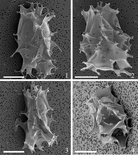
Plate 9. 1–4. Scanning electron micrographs of lateral and dorsal views of four different specimens of Spiniferites elongatus from the Barents Sea with significant variation in the elevation of sutural crests, showing the position of sulcal plate boundaries and a reduced archaeopyle corresponding to 3′′. Scale bars = 10 µm.

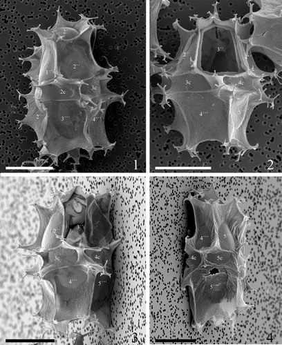
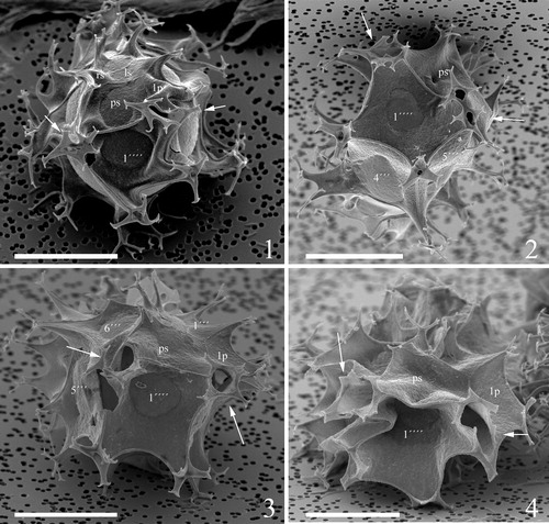
Plate 10. 1–4. Scanning electron micrographs of antapical views of four different specimens of Spiniferites elongatus from the Barents Sea with significant variation in the elevation of sutural crests, showing the antapical plate configuration with significant variation in fusion of ventral antapical multifurcate processes, indicated by white arrows on all specimens. 1p = posterior intercalary plate, ls = left sulcal plate, ps = posterior sulcal plate, rs = right sulcal plate. Scale bars = 10 µm.

Reid PC. 1974. Gonyaulacacean dinoflagellate cysts from the British Isles. Nova Hedwigia. 25:579–637.

 Google Scholar

Ellegaard M, Daugbjerg N, Rochon A, Lewis J, Harding I. 2003. Morphological and LSU rDNA sequence variation within the Gonyaulax spinifera-Spiniferites group (Dinophyceae) and proposal of G. elongata comb. nov. and G. membranacea comb. nov. Phycologia. 42(2):151–164.

 Web of Science ®Google Scholar

Matsuoka K. 1983. Late Cenozoic dinoflagellates and acritarchs in the Niigata district, central Japan. Palaeontogr Abteilung B. 187:89–154.

 Google Scholar

Harland R, Sharp J. 1986. Elongate Spiniferites cysts from North Atlantic bottom sediments. Palynology. 10(1):25–34.

 Google Scholar

Evitt WR. 1985. Sporopollenin dinoflagellate cysts: their morphology and interpretation. AASP Monograph Series. 1:333.

 Google Scholar