Predicting future failures in generalized order statistics and related models

Figures & data

Figure 1. Absolute value differences between generalized order statistics and predictions with known parameter ϑ based on the median (black circles) or the mean (red squares) and with unknown parameter ϑ based on the median (blue triangles) or the mean (green stars) from the simulated sample in Example 5.1 with m = 20, and s−r = 1 (left). Predictions (red) for $X_{(s)}^{\ast }$ from $X_{(r)}^{\ast }$ for m = 20, s−r = 1, for the exponential distribution in Example 5.1. The black points are the observed values and the blue lines are the limits for the $50\mathrm{\%}$ (continuous lines) and the $90\mathrm{\%}$ (dashed lines) prediction intervals (right).

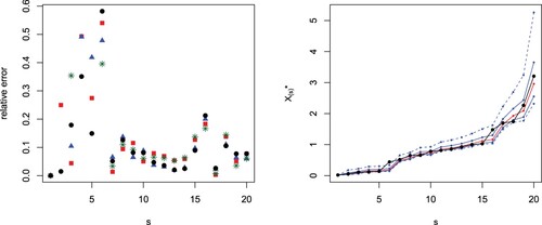
Figure 2. Absolute value differences between generalized order statistics and predictions with known parameter ϑ based on the median (black circles) or the mean (red squares) and with unknown parameter ϑ based on the median (blue triangles) or the mean (green stars) from the simulated sample in Example 5.1 with m = 20, and s−r = 2 (left). Predictions (red) for $X_{(s)}^{\ast }$ from $X_{(r)}^{\ast }$ for m = 20, s−r = 2, for the exponential distribution in Example 5.1. The black points are the observed values and the blue lines are the limits for the $50\mathrm{\%}$ (continuous lines) and the $90\mathrm{\%}$ (dashed lines) prediction intervals (right).

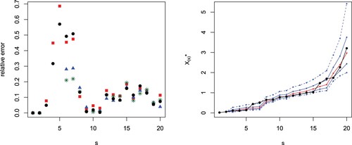
Table 1. Predicted values based on the median ${\hat{X}}_{(s)}^{\ast }$ from $X_{(r)}^{\ast }$ assuming known ϑ in Example 5.1 for some choices of r and s such that $s-r\ge 2$. In the bottom line we provide the exact values.

	s
r	3	6	9	11	14	18	20
1	0.10948	0.29518	0.52390	0.71184	1.08320	1.99725	3.34785
2		0.27948	0.50814	0.69607	1.06741	1.98148	3.33210
5			0.41177	0.59962	0.97092	1.88498	3.23571
7			0.65108	0.83860	1.20979	2.12384	3.47464
10					1.22134	2.13525	3.48622
12					1.08445	1.99768	3.34884
15						1.71923	3.07052
$X_{(s)}^{\ast }$	0.11512	0.44063	0.65636	0.81377	1.00213	1.74417	3.20779

Table 2. Number of exact values out of the 50% and $90\mathrm{\%}$ prediction intervals with fixed r in the sample of size 20 considered in Example 5.1.

r	1	2	3	4	5	6	7	8	9	10	11	12	13	14	15	16	17	18
$50\mathrm{\%}$	5	6	6	6	5	4	3	5	3	5	3	1	1	0	1	1	0	0
$90\mathrm{\%}$	0	0	0	1	2	0	0	1	0	1	0	0	0	0	0	0	0	0
out-of	18	17	16	15	14	13	12	11	10	9	8	7	6	5	4	3	2	1

Table 3. Predicted values based on the mean ${\tilde{X}}_{(s)}^{\ast }$ from $X_{(r)}^{\ast }$ assuming known ϑ in Example 5.1 for some choices of r and s such that $s-r\ge 2$. In the bottom line we provide the exact values.

	s
r	3	6	9	11	14	18	20
1	0.12407	0.30639	0.52953	0.71186	1.06853	1.91583	3.01444
2		0.29241	0.51555	0.69787	1.05455	1.90185	3.00046
5			0.42581	0.60813	0.96481	1.81211	2.91072
7			0.67079	0.85312	1.20979	2.05709	3.15570
10					1.23466	2.08196	3.18057
12					1.11120	1.95850	3.05711
15						1.71921	2.81782
$X_{(s)}^{\ast }$	0.11512	0.44063	0.65636	0.81377	1.00213	1.74417	3.20779

Table 4. Predicted values based on the median ${\hat{X}}_{(s)}^{\ast }$ from $X_{(r)}^{\ast }$ assuming unknown ϑ in Example 5.1 for some choices of r and s such that $s-r\ge 2$. In the bottom line we provide the exact values.

	s
r	3	6	9	11	14	18	20
1	0.26130	0.75758	1.36886	1.87115	2.86363	5.30647	8.91601
2		0.46867	0.89091	1.23794	1.92367	3.61162	6.10569
5			0.68207	1.51595	1.79355	3.61050	6.29546
7			0.63285	0.79429	1.11440	1.90267	3.06785
10					1.17024	1.97769	3.17129
12					1.08362	1.99348	3.33965
15						1.81067	3.34024
$X_{(s)}^{\ast }$	0.11512	0.44063	0.65636	0.81377	1.00213	1.74417	3.20779

Table 5. Predicted values based on the mean ${\tilde{X}}_{(s)}^{\ast }$ from $X_{(r)}^{\ast }$ assuming unknown ϑ in Example 5.1 for some choices of r and s such that $s-r\ge 2$. In the bottom line we provide the exact values.

	s
r	3	6	9	11	14	18	20
1	0.30029	0.78755	1.38392	1.87118	2.82442	5.08887	8.02497
2		0.49254	0.90460	1.24128	1.89992	3.46456	5.49328
5			0.70998	1.07240	1.78139	3.46564	5.64945
7			0.64958	0.80681	1.11440	1.84510	2.79253
10					1.18201	1.93061	2.90124
12					1.11027	1.95444	3.04900
15						1.81065	3.05419
$X_{(s)}^{\ast }$	0.11512	0.44063	0.65636	0.81377	1.00213	1.74417	3.20779

Figure 3. Absolute value differences between generalized order statistics and predictions with known parameter ϑ based on the median (black circles) or the mean (red squares) and with unknown parameter ϑ based on the median (blue triangles) or the mean (green stars) from the simulated sample in Example 5.2 with m = 20, and s−r = 1 (left). Predictions (red) for $X_{(s)}^{\ast }$ from $X_{(r)}^{\ast }$ for m = 20, s−r = 1, for the exponential distribution in Example 5.2. The black points are the observed values and the blue lines are the limits for the $50\mathrm{\%}$ (continuous lines) and the $90\mathrm{\%}$ (dashed lines) prediction intervals (right).

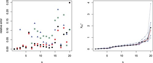
Figure 4. Absolute value differences between generalized order statistics and predictions with known parameter ϑ based on the median (black circles) or the mean (red squares) and with unknown parameter ϑ based on the median (blue triangles) or the mean (green stars) from the simulated sample in Example 5.2 with m = 20, and s−r = 2 (left). Predictions (red) for $X_{(s)}^{\ast }$ from $X_{(r)}^{\ast }$ for m = 20, s−r = 2, for the exponential distribution in Example 5.2. The black points are the observed values and the blue lines are the limits for the $50\mathrm{\%}$ (continuous lines) and the $90\mathrm{\%}$ (dashed lines) prediction intervals (right).

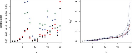
Table 6. Predicted values based on the median ${\hat{X}}_{(s)}^{\ast }$ from $X_{(r)}^{\ast }$ assuming known ϑ in Example 5.2 for some choices of r and s such that $s-r\ge 2$. In the bottom line we provide the exact values.

	s
r	3	6	9	11	14	18	20
1	0.03784	0.10242	0.18274	0.24962	0.38469	0.74947	1.76574
2		0.09698	0.17730	0.24419	0.37921	0.74401	1.76033
5			0.14382	0.21063	0.34566	0.71052	1.72696
7			0.22727	0.29398	0.42898	0.79377	1.81041
10					0.43295	0.79774	1.81470
12					0.38377	0.74831	1.76561
15						0.64459	1.66292
$X_{(s)}^{\ast }$	0.03980	0.15333	0.22902	0.28495	0.35364	0.64422	1.84707

Table 7. Number of exact values out of the 50% and $90\mathrm{\%}$ prediction intervals with fixed r in the sample of size 20 considered in Example 5.2.

r	1	2	3	4	5	6	7	8	9	10	11	12	13	14	15	16	17	18
$50\mathrm{\%}$	6	6	7	6	5	4	4	5	3	5	3	1	1	0	1	1	0	0
$90\mathrm{\%}$	0	0	0	1	2	0	0	1	0	1	0	0	0	0	0	0	0	0
out-of	18	17	16	15	14	13	12	11	10	9	8	7	6	5	4	3	2	1

Table 8. Predicted values based on the mean ${\tilde{X}}_{(s)}^{\ast }$ from $X_{(r)}^{\ast }$ assuming known ϑ in Example 5.2 for some choices of r and s such that $s-r\ge 2$. In the bottom line we provide the exact values.

	s
r	3	6	9	11	14	18	20
1	0.04352	0.10822	0.18856	0.25540	0.39037	0.75394	1.67024
2		0.10309	0.18344	0.25028	0.38524	0.74882	1.66511
5			0.15114	0.21798	0.35295	0.71652	1.63281
7			0.23559	0.30243	0.43739	0.80097	1.71726
10					0.44391	0.80748	1.72377
12					0.39730	0.76087	1.67716
15						0.66556	1.58185
$X_{(s)}^{\ast }$	0.03980	0.15333	0.22902	0.28495	0.35364	0.64422	1.84707

Table 9. Predicted values based on the median ${\hat{X}}_{(s)}^{\ast }$ from $X_{(r)}^{\ast }$ assuming unknown ϑ in Example 5.2 for some choices of r and s such that $s-r\ge 2$. In the bottom line we provide the exact values.

	s
r	3	6	9	11	14	18	20
1	0.09034	0.26294	0.47758	0.65532	1.01731	1.99221	4.70826
2		0.16271	0.31103	0.43456	0.68389	1.35753	3.23429
5			0.23866	0.37148	0.63988	1.36515	3.38562
7			0.22076	0.27829	0.39471	0.70930	1.58603
10					0.41442	0.73671	1.63520
12					0.38346	0.74667	1.76021
15						0.68179	1.83447
$X_{(s)}^{\ast }$	0.03980	0.15333	0.22902	0.28495	0.35364	0.64422	1.84707

Table 10. Predicted values based on the mean ${\tilde{X}}_{(s)}^{\ast }$ from $X_{(r)}^{\ast }$ assuming unknown ϑ in Example 5.2 for some choices of r and s such that $s-r\ge 2$. In the bottom line we provide the exact values.

	s
r	3	6	9	11	14	18	20
1	0.10551	0.27842	0.49316	0.67179	1.03250	2.00417	4.45301
2		0.17339	0.32236	0.44579	0.69502	1.36640	3.05845
5			0.25322	0.38608	0.65436	1.37707	3.19847
7			0.22793	0.28557	0.40196	0.71550	1.50570
10					0.42410	0.74532	1.55487
12					0.39695	0.75918	1.67209
15						0.70552	1.74270
$X_{(s)}^{\ast }$	0.03980	0.15333	0.22902	0.28495	0.35364	0.64422	1.84707

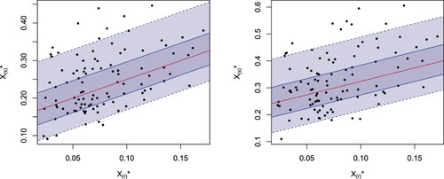
Figure 5. Scatterplots of a simulated sample of size N = 100 from $(X_{(r)}^{\ast },X_{(s)}^{\ast })$ for $m=20$, r = 4 and s = 5 (left) and r = 4, s = 6 (right) for the exponential distribution in Example 5.3 jointly with the theoretical median regression curves (red) and $50\mathrm{\%}$ (dark grey) and $90\mathrm{\%}$ (light grey) prediction bands.

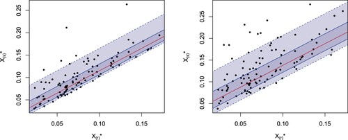
Figure 6. Scatterplots of a simulated sample of size N = 100 from $(X_{(r)}^{\ast },X_{(s)}^{\ast })$ for $m=20$, r = 4 and s = 10 (left) and r = 4, s = 12 (right) for the exponential distribution in Example 5.3 jointly with the theoretical median regression curves (red) and $50\mathrm{\%}$ (dark grey) and $90\mathrm{\%}$ (light grey) prediction bands.