An adaptive patch approximation algorithm for bicriteria convex mixed-integer problems

Figures & data

Figure 1. An illustration of three patches in objective space.

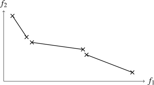
Figure 2. Illustration of the ideal point and nadir point in objective space. The thick curve and the dotted point represent the set of nondominated objective vectors.

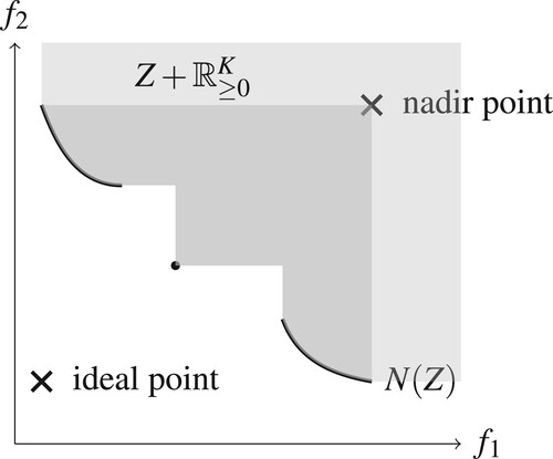
Figure 3. Illustration of two segment patches in a two-dimensional objective space. The patch s corresponds to the discrete assignment d and has endpoints given as $\left(X_1\right(s),Y_1(s\left)\right)$ and $\left(X_2\right(s),Y_2(s\left)\right)$. Another patch corresponds to a different discrete assignment $d^{\prime }$. The grey background represents the upper set $Z+{\mathbb{R}}_{\ge 0}^2$ of attainable objective vectors.

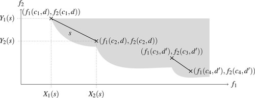
Figure 4. Illustration of ε-indicator value and difference volume for an approximation A (thick black line) of the true Pareto frontier Z (the boundary of the shaded area). The darker shaded area represents the difference volume ${\delta }_{\mathrm{vol}}(Z,A)$. The ε-indicator value ${ϵ}_d(Z,A)$ is illustrated with the dotted line.

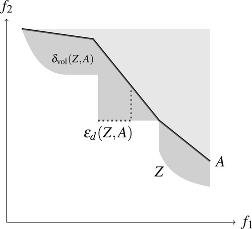
Figure 5. Illustration of the monotone lower envelope m (solid line) for a set of segments (dashed). The dotted line shows the difference in value for the monotone lower envelope m and the standard lower envelope ℓ at the position $x^{\prime }$.

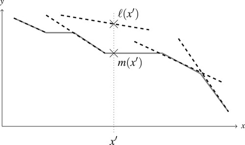
Figure 6. Illustration of the partition of objective space into regions induced by the segments of the approximation.

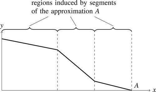
Figure 7. A new segment patch p (dotted) is found w.r.t. the reference segment m. Two cases can arise when the new patch p is inserted into the old monotone lower envelope (solid). In both cases, only four segments are updated or newly created in the new monotone lower envelope (dashed). (a) New segment above reference segment. (b) New segment below reference segment.

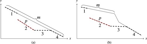
Figure 8. Approximation of the logarithm (solid line) via linear inequalities (dashed lines). The shown plot corresponds to the choice ${\text{β}}^{\prime }=0.2$. With the tangents through the three points $x_0$, $x_1$, $x_2$ we obtain an upper approximation of $\ln \left(x\right)$ with an additive error of at most ${\text{β}}^{\prime }=0.2$ for the interval $[{\delta }_0,1]=[z_3,1]\approx [0.022,1]$ which is attained at the points $z_1$, $z_2$ and $z_3$.

Figure 9. Illustration of the approximations of the Pareto frontier generated by our algorithm for problem (T4). The approximation created after iteration 5 has a difference volume of 0.038, after 10 iterations the difference volume has already reached 0.018, while with 60 iterations, the difference volume is smaller than 0.001.

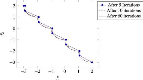
Table 1. Comparison of the required number of steps on instance (T4) for our algorithm with the required number of branching nodes reported in [2, Table 1].

Number of integer variables	1	2	3
Number of iterations by our algorithm until ${\delta }_{\mathrm{vol}}\le {10}^{-3}$	36	95	70
Number of branching nodes generated by the algorithm in [2]	749	3683	19,127

Note that the used stopping criteria are not equivalent but correspond to roughly similar levels of approximation quality.

Figure 10. Illustration of the approximations of the Pareto frontier generated by our algorithm for problem (T6). The approximation created after iteration 5 has a difference volume of 0.025, after 10 iterations the difference volume has already reached 0.009, and after 36 iterations, the difference volume is smaller than 0.001.

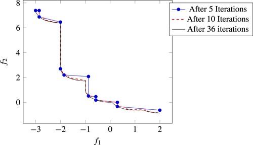
Figure 11. Dependence of the approximation quality on the number of iterations. Average over 10 instances of the benchmark problem by Mavrotas of Appendix 5 with 320 variables.

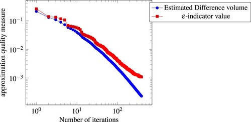
Figure 12. Heatmap of the approximation quality reached after a given number of iterations for varying instance sizes of the benchmark of Mavrotas. The shade corresponds to the logarithm to the base 10 of the respective approximation quality measure. (a) Difference Volume, (b) e-indicator value.

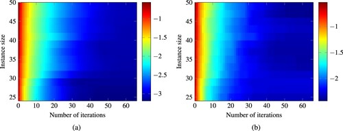
Figure 13. Comparison of the required number of MIP solutions by several algorithms for the benchmark problems by Mavrotas and Diakoulaki [15]. The instance size corresponds to the total number of variables.

Figure 14. Comparison of running times required by several algorithms for the benchmark problems by Mavrotas and Diakoulaki [15]. The instance size corresponds to the total number of variables.

Figure 15. Heatmap of the approximation quality reached after a given number of iterations for varying instance sizes of the capacitated facility location benchmark. The shade corresponds to the logarithm to the base 10 of the respective approximation quality measure. (a) Difference Volume, (b) e-indicator value.

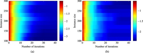
Figure 16. Heatmap of the approximation quality after a given number of iterations for varying instance sizes of the biobjective assignment benchmark. The shade corresponds to the logarithm to the base 10 of the respective approximation quality measure. (a) Difference Volume, (b) e-indicator value.

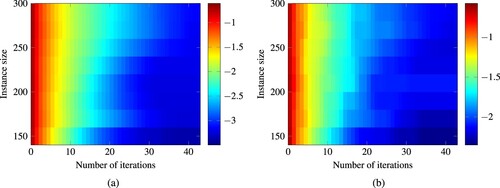
Figure 17. Comparison of the running times of [16, Figure 11], using the best-performing variant BOBB-32, with running times for our algorithm. Note that for the instance size of 2025, the algorithm of [16] reaches its time limit of 300 s.

de Santis M, Eichfelder G, Niebling J, et al. Solving multiobjective mixed integer convex optimization problems. SIAM J Optim. 2020;30(4):3122–3145.

 Web of Science ®Google Scholar

Mavrotas G, Diakoulaki D. A branch and bound algorithm for mixed zero-one multiple objective linear programming. Eur J Oper Res. 1998;107(3):530–541.

 Web of Science ®Google Scholar

Stidsen T, Andersen KA, Dammann B. A branch and bound algorithm for a class of biobjective mixed integer programs. Manage Sci. 2014;60(4):1009–1032.

 Web of Science ®Google Scholar