Portfolio reshaping under 1st-order stochastic dominance constraints by the exact penalty function methods

Figures & data

Figure 1. Possible (disconnected and non-convex) shapes of feasible sets under 1st-order SDC ($x_{\mathit{ref}}=(x_1=0.31,x_2=0.69)$, $\delta =0.05,0,0$).

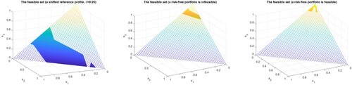
Figure 2. Illustration of the smoothing method performance on two asset (1,2) portfolio selection. Examples of the trajectories of the method for different discontinuous penalties. $x_{\mathit{ref}}=(x_1=0.3,x_2=0.7)$, $\delta =0.05$.

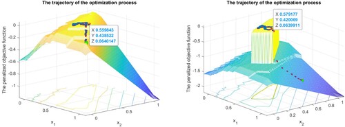
Figure 3. Illustration of the smoothing method performance on two asset (4,9) portfolio selection. Example of the trajectory of the method for non-connected feasible set. $x_{\mathit{ref}}=(x_4=0.3,x_9=0.7)$, $\delta =0.05$. The green is the starting point, the red is the final one.

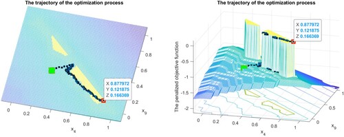
Figure 4. Profiles of optimal 3 component portfolios: maximizing the tail returns under the risk-return lower bound. Discontinuous penalties. 1) Optimal average return. 2) Optimal ${\mathrm{V}@\mathrm{R}}_{40\mathrm{\%}}$. 3) Optimal ${\mathrm{AV}@\mathrm{R}}_{40\mathrm{\%}}$; cf. Table 1.

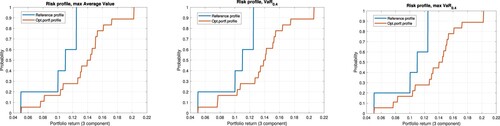
Figure 5. Profiles of optimal 3 component portfolios: maximizing the tail returns under the risk-return lower bound. Analytical projective penalties. (1) Optimal average return. (2) Optimal ${\mathrm{V}@\mathrm{R}}_{0.4}$. (3) Optimal ${\mathrm{AV}@\mathrm{R}}_{0.4}$. See Table 2.

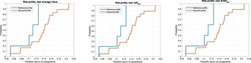
Table 1. Optimal 3 component portfolios, discontinuous penalties: (1) Max mean; (2) Max $\mathrm{V}@\mathrm{R}$; (3) Max $\mathrm{AV}@\mathrm{R}$.

Objective	Value	$x_4$	$x_9$	$x_{10}$
(1) Mean	0.1351	0.1229	0.0085	0.8675
(2) ${\mathrm{V}@\mathrm{R}}_{0.4}$	0.1344	0.1313	0.0001	0.8670
(3) ${\mathrm{AV}@\mathrm{R}}_{0.4}$	0.1554	0.1219	0.0105	0.8675

Note: See Figure 4.

Table 2. Optimal 3 component portfolios, analytical projection: (1) Max mean. (2) Max ${\mathrm{V}@\mathrm{R}}_{40\mathrm{\%}}$. (3) Max ${\mathrm{AV}@\mathrm{R}}_{40\mathrm{\%}}$.

Objective	Value	$x_4$	$x_9$	$x_{10}$
(1) Mean	0.1357	0.1308	0.0009	0.8683
(2) ${\mathrm{V}@\mathrm{R}}_{40\mathrm{\%}}$	0.1527	0.1298	0.0000	0.8702
(3) ${\mathrm{AV}@\mathrm{R}}_{40\mathrm{\%}}$	0.1709	0.1313	0.0004	0.8684

Note: See Figure 5.

Figure 6. Profiles of optimal 3 component portfolios: maximizing the tail returns under the risk-return lower bound. Analytical projective penalties. (1) Optimal average return. (2) Optimal ${\mathrm{V}@\mathrm{R}}_{70\mathrm{\%}}$. (3) Optimal ${\mathrm{AV}@\mathrm{R}}_{70\mathrm{\%}}$. See Table 3.

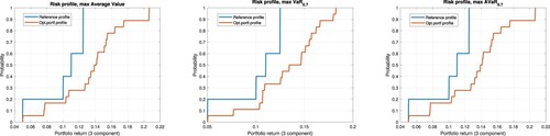
Figure 7. Profiles of optimal 10 component portfolios: maximizing the tail returns under the risk-return lower bound. Analytical projective penalties. (1) optimal average return; (2) optimal ${\mathrm{V}@\mathrm{R}}_{70\mathrm{\%}}$; (3) optimal ${\mathrm{AV}@\mathrm{R}}_{70\mathrm{\%}}$; cf. Tables 4 and 5.

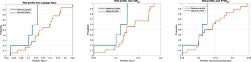
Table 3. Optimal 3 component portfolios, analytical projection: (1) Max mean. (2) Max $\mathrm{V}@\mathrm{R}$. (3) Max $\mathrm{AV}@\mathrm{R}$.

Objective	Value	$x_4$	$x_9$	$x_{10}$
(1) Mean	0.1357	0.1308	0.0009	0.8683
(2) ${\mathrm{V}@\mathrm{R}}_{70\mathrm{\%}}$	0.1549	0.0797	0.0557	0.8643
(3) ${\mathrm{AV}@\mathrm{R}}_{70\mathrm{\%}}$	0.1709	0.1315	0.0001	0.8684

Note: See Figure 6.

Table 4. Optimal 10 component portfolios, analytical projection: (1) Max mean. (2) Max $\mathrm{V}@\mathrm{R}$. (3) Max $\mathrm{AV}@\mathrm{R}$.

Objective	Value	$x_4$	$x_9$	$x_{10}$
(1) Mean	0.1380	0.0126	0.0022	0.8615
(2) ${\mathrm{V}@\mathrm{R}}_{70\mathrm{\%}}$	0.1728	0.0006	0.0425	0.8418
(3) ${\mathrm{AV}@\mathrm{R}}_{70\mathrm{\%}}$	0.1901	0.0126	0.0002	0.8490

Note: See Figure 7.

Table 5. The optimal 10 component portfolio.

Portfolio	$x_1$	$x_2$	$x_3$	$x_4$	$x_5$	$x_6$	$x_7$	$x_8$	$x_9$	$x_{10}$
Mean	.0013	.0001	.0059	.0126	.1011	.0008	.0031	.0117	.0022	.8615
${\mathrm{V}@\mathrm{R}}_{0.7}$	.0029	.0103	.0137	.0006	.0512	.0128	.0038	.0202	.0425	.8418
${\mathrm{AV}@\mathrm{R}}_{0.7}$	.0001	.0001	.0201	.0126	.0083	.0005	.0001	.1090	.0002	.8490

Table A1. Return data set from [62, Table 1, page 13], with artificial bond column.

Year	Am.T.	A.T.&T.	U.S.S.	G.M.	A.T.&Sfe	C.C.	Bdn.	Frstn.	S.S.	Bond
1937	−0.305	−0.173	−0.318	−0.477	−0.457	−0.065	−0.319	−0.400	−0.435	0.125
1938	0.513	0.098	0.285	0.714	0.107	0.238	0.076	0.336	0.238	0.125
1939	0.055	0.200	−0.047	0.165	−0.424	−0.078	0.381	−0.093	−0.295	0.125
1940	−0.126	0.030	0.104	−0.043	−0.189	−0.077	−0.051	−0.090	−0.036	0.125
1941	−0.280	−0.183	−0.171	−0.277	0.637	−0.187	0.087	−0.400	−0.240	0.125
1942	−0.003	0.067	−0.039	0.476	0.865	0.156	0.262	1.113	0.126	0.125
1943	0.428	0.300	0.149	0.225	0.313	0.351	0.341	0.580	0.639	0.125
1944	0.192	0.103	0.260	0.290	0.637	0.233	0.227	0.473	0.282	0.125
1945	0.446	0.216	0.419	0.216	0.373	0.349	0.352	0.229	0.578	0.125
1946	−0.088	−0.046	−0.078	−0.272	−0.037	−0.209	0.153	−0.126	0.289	0.125
1947	−0.127	−0.071	0.169	0.144	0.026	0.355	−0.099	0.009	0.184	0.125
1948	−0.015	0.056	−0.035	0.107	0.153	−0.231	0.038	0.000	0.114	0.125
1949	0.305	0.038	0.133	0.321	0.067	0.246	0.273	0.223	−0.222	0.125
1950	−0.096	0.089	0.732	0.305	0.579	−0.248	0.091	0.650	0.327	0.125
1951	0.016	0.090	0.021	0.195	0.040	−0.064	0.054	−0.131	0.333	0.125
1952	0.128	0.083	0.131	0.390	0.434	0.079	0.109	0.175	0.062	0.125
1953	−0.010	0.035	0.006	−0.072	−0.027	0.067	0.210	−0.084	−0.048	0.125
1954	0.154	0.176	0.908	0.715	0.469	0.077	0.112	0.756	0.185	0.125

Markowitz HM. Portfolio selection. efficient diversification of investments. New York: John Wiley & Sons, Chapman & Hall; 1959.

 Google Scholar