Luminescent, Redox-Active Dithiolatobis(imine)platinum(II) Divergent Complexes with Exchangeable Imine Ligands: An Experimental/Computational Study Versus Their Diiminedithiolatoplatinum(II) Convergent Congeners

Figures & data

Table 1 Crystallographic data for compounds 1 and 3•C₃H₆O•2H₂O

	1	3•C3H6O•2H2O
Formula	C12H8N6PtS2	C17H22N6O3PtS2
space group	P-1	P-1
a, Å	8.8424(18)	9.1050(18)
b, Å	9.0440(18)	11.153(2)
c, Å	10.693(2)	11.709(2)
α, deg	86.08(3)	80.66(3)
β, deg	78.61(3)	74.95(3)
γ, deg	64.08(3)	85.53(3)
V, Å^3	753.8(3)	1129.9(4)
Z	2	2
T, K	295	291
D, g/cm	2.1826	1.8152
R1	0.0187	0.0468
R1 (all data)	0.0218	0.0655
wR2 (all data)	0.0458	0.0993
GOF	1.040	0.9897

Scheme 1 (a) Syntheses of 1 (L = pyz) and 2 (L = 4,4ʹ-bpy) from [Pt(κ¹-NN)₄]²⁺ and (b) subsequent exchange of pyz ligands in 1 to form 2 or 3 (L = 4-ap)).

Figure 1 ¹H NMR spectra of Pt(pyz)₂(mnt), 1 (a), Pt(4-ap)₂(mnt), 3 (b) and Pt(4,4ʹ-bpy)₂(mnt), 2 (c).

Table 2 Select bond lengths, angles, and torsion angles for Pt(pyz)₂(mnt), 1, and Pt(4-ap)₂(mnt), 3

Bond Length (Å), 1			Angle (°), 1
	Experimental	Theoretical		Experimental	Theoretical
Pt1—S2	2.2460(12)	2.3084	S1—Pt1—S2	90.97(3)	90.32
Pt1—S1	2.2429(11)	2.3804	N5—Pt1—S2	90.46(7)	89.30
Pt1—N5	2.077(3)	2.1268	N5—Pt1—S1	178.22(7)	179.18
Pt1—N3	2.078(3)	2.1270	N3—Pt1—N5	88.36(10)	91.09
S1—C1	1.739(3)	1.7588	C1—S1—Pt1	102.54(12)	102.49
S2—C2	1.739(3)	1.7588	C2—C1—S1	122.1(2)	122.35
N1—C3	1.150(4)	1.1874	Torsion Angle (°), 1
C2—C4	1.431(4)	1.4506		Experimental	Theoretical
C2—C1	1.360(5)	1.3915	PtS2C2—N3 Ring	49.24(12)	54.03
C4—N2	1.141(4)	1.1873	PtS2C2—N5 Ring	61.33(12)	54.07
C3—C1	1.429(5)	1.4506	N3 Ring—N5 Ring	72.50(13)	70.97
Bond Length (Å), 3			Angle (°), 3
	Experimental	Theoretical		Experimental	Theoretical
Pt1—S2	2.249(2)	2.3103	S1—Pt1—S2	90.89(7)	90.52
Pt1—S1	2.2446(18)	2.3103	N5—Pt1—S1	91.25(16)	89.89
Pt1—N5	2.049(6)	2.1312	N5—Pt1—S2	175.81(17)	179.01
Pt1—N3	2.062(5)	2.1312	N3—Pt1—N5	86.6(2)	89.90
S1—C2	1.741(7)	1.7595	C1—S2—Pt1	102.1(2)	102.28
S2—C1	1.737(7)	1.7585	C1—C2—S1	122.6(5)	122.46
N1—C3	1.154(10)	1.1880		Torsion Angle (°), 3
C2—C4	1.435(10)	1.4506		Experimental	Theoretical
C2—C1	1.342(9)	1.3935	PtS2C2—N3 Ring	56.9(2)	56.03
C4—N2	1.132(9)	1.1880	PtS2C2—N5 Ring	60.8(2)	56.92
C3—C1	1.413(10)	1.4506	N3 Ring—N5 Ring	74.0(2)	74.55

Table 3 Select calculated bond lengths, angles and torsion angles for Pt(4,4ʹ-bpy)₂(mnt), 2

Bond Length (Å), 2		Angle (°), 2
Pt1—S2	2.309	S1—Pt1—S2	90.45
Pt1—S1	2.309	N5—Pt1—S1	89.53
Pt1—N5	2.131	N5—Pt1—S2	179.31
Pt1—N3	2.131	N3—Pt1—N5	90.49
S1—C2	1.759	C1—S2—Pt1	102.37
S2—C1	1.759	C1—C2—S1	122.41
N1—C3	1.188	Torsion Angle (°), 2
C2—C1	1.392	PtS2C2—N3 Ring	56.30
C4—N2	1.188	PtS2C2—N5 Ring	56.30
C3—C1	1.451	N3 Ring—N5 Ring	73.91

Figure 2 Crystal structures (ellipsoids at 50%) of the H-bonded quadrangle containing two units of Pt(4-ap)₂(mnt), 3, and two water molecules. Other solvent molecules omitted for clarity (top) and Pt(pyz)₂(mnt), 1, (bottom).

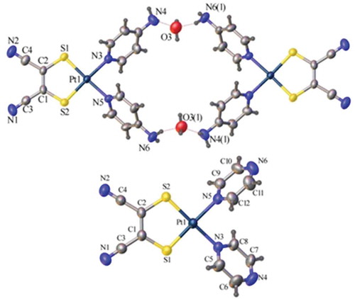
Figure 3 Crystal structures (ellipsoids at 50%) of 1 (top) and 3 (bottom) showing head-to-tail packing. H-atoms and solvent molecules omitted for clarity.

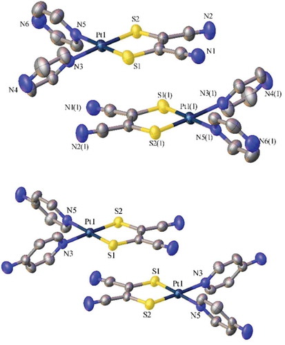
Table 4 Redox potentials for compounds 1–3 at a scan rate of 0.1 V/s. *Quasi-reversible while others are irreversible. All E_c and E_a values represent peak potentials.

Compound (Solvent)	Ec (V)	Ea (V)
1 (THF)	−1.37, −1.77	1.37
2 (DMF)	−1.30*, −1.41*	1.23
3 (MeCN)	−1.42, −1.65	1.06*, 1.21*

Table 5 Comparison of experimental and calculated reduction/oxidation potentials for 1, 2, 3, and Pt(2,2ʹ-bpy)(mnt). E^abs_exp was calculated according to E^abs = E_exp + 4.696 V to convert from a Ag/AgCl reference electrode to vacuum and E^abs_calc = ΔG_sol/nF where ΔG_sol = ΔG°^x_sol – ΔG^red_sol. Experimental values for Pt(2,2ʹ-bpy)(mnt) taken from ^[50]

	Oxidation		Reduction
	E^abscalc (V)	E^absexp. (V)	E^abscalc (V)	E^absexp. (V)
1 (in THF)	5.60	6.07	2.94	3.33
2 (in DMF)	5.00	5.93	3.32	3.40
3 (in MeCN)	5.20	5.91	2.47	3.28
Pt(2,2ʹ-bpy)(mnt) (in DMF)	5.39	5.76	3.49	3.29

Figure 4 SOMO–1 (top) and SOMO (bottom) contours for 1 (left), 2 (middle), and 3 (right) (plotted with an isovalue of 0.02), supporting assignment of oxidation and reduction processes.

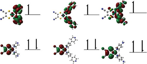
Figure 5 Cyclic voltammagram of 3 with five complete cycles from 0 to 1.5 V (red) and one cycle from 0 to 0.9 V (blue), indicating dependence of cathodic peak on oxidations at higher potential. Performed in acetonitrile using 0.1 M [n-Bu₄N][PF₆] electrolyte with a scan rate of 0.1 V/s.

Figure 6 Cyclic voltammagrams of 3 with increasing scan rate showing a negative shift in the oxidation potential dependent on scan rate.

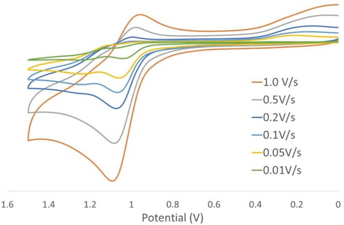
Figure 7 Cyclic voltammagram of 3 with increasing concentrations (0.2 mM, 0.4 mM, and 0.8 mM) indicating concentration dependence of cathodic peak at 0.32 V. Performed in acetonitrile using 0.1 M [n-Bu₄N][PF₆] electrolyte with a scan rate of 0.1 V/s.

Figure 8 Electronic adsorption spectra of compounds 1–3 exhibiting diimine-based π-π* absorptions in the mid-UV region and tunable MMLL’CT in the near-UV extending into the visible region.

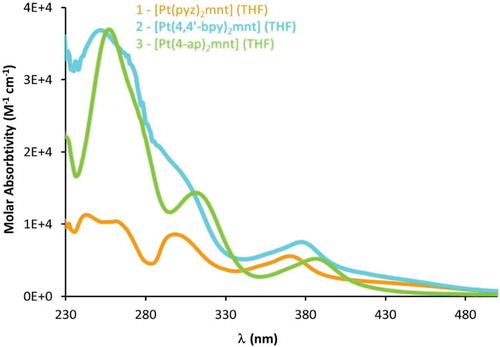
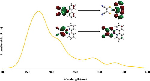
Figure 9 Calculated absorption spectra of 1 (a), 2 (b), and 3 (c) with orbital contours for the transition with the highest oscillator strength.

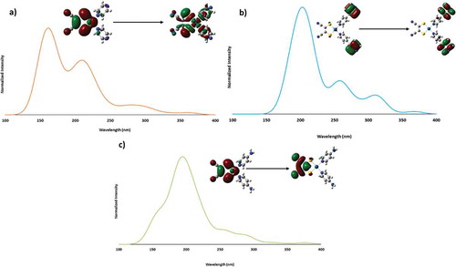
Table 6 Summary of lifetime data for frozen glassy solutions of 1 (10⁻³ M), 2 (10⁻⁴ M), and 3 (10⁻³ M) in acetone

Pt(pyz)2(mnt)		Pt(4,4`-bpy)2(mnt)		Pt(4-ap)2(mnt)
λex/λem	LT (μs)	λex/λem	LT (μs)	λex/λem	LT (μs)
314–622	37.77 ± 3.069e-1	318–623	31.72 ± 3.773e-1	315–630	25.04 ± 3.068e-1
314–672	36.84 ± 4.470e-1	318–650	30.27 ± 2.015e-1	315–660	23.66 ± 2.343e-1
314–730	38.36 ± 3.547e-1	318–675	30.89 ± 3.560e-1	315–685	25.04 ± 2.607e-1
370–622	38.35 ± 2.177e-1	390–623	32.99 ± 2.380e-1	315–710	24.19 ± 1.532e-1
370–672	36.58 ± 1.750e-1	390–650	29.97 ± 2.767e-1	377–630	26.7 ± 8.692e-2
370–730	34.61 ± 7.300e-1	390–675	32.3 ± 2.413e-1	377–660	25.13 ± 1.261e-1
420–622	38.33 ± 2.151e-1	430–623	32.16 ± 1.318e-1	377–685	26.36 ± 1.688e-1
420–672	36.15± 3.490e-1	430–650	28.32 ± 2.258e-1	406–630	25.94 ± 1.018e-1
420–730	37.05± 2.947e-1	430–675	30.18 ± 1.939e-1	406–660	24.56 ± 1.186e-1
				406–685	26.35 ± 1.080e-1

Table 7 Summary of lifetime data for solid samples of 1, 2, and 3 at 77 K

Pt(pyz)2(mnt)		Pt(4,4ʹ-bpy)2(mnt)		Pt(4-ap)2(mnt)
λex/λem	LT (μs)	λex/λem	LT (μs)	λex/λem	LT (μs)
360–635	9.208 ± 1.621e-1	365–630	14.4 ± 1.386e-1	370–665	7.834 ± 1.281e-1
360–660	8.818 ± 2.002e-1	365–660	15.03 ± 1.031e-1	370–700	7.743 ± 1.377e-1
360–695	10.48 ± 8.543e-2	365–695	13.35 ± 6.438e-2	370–720	8.343 ± 1.484e-1
360–715	10.68 ± 8.580e-2	365–715	13.4 ± 1.283e-1	370–735	8.216 ± 1.184e-1
360–732	9.991 ± 1.590e-1	365–735	14.49 ± 1.142e-1	370–740	7.735 ± 9.914e-2
360–750	9.879 ± 1.880e-1	365–767	13.33 ± 1.545e-1	370–768	7.21 ± 1.600e-1
450–635	9.76 ± 1.677e-1	437–630	14.16 ± 1.170e-1	410–665	7.953 ± 9.414e-2
450–660	10.57 ± 9.549e-2	437–660	14.21 ± 1.131e-1	410–700	8.313 ± 1.667e-1
450–695	10.67 ± 8.082e-2	437–695	13.15 ± 9.819e-2	410–720	7.781 ± 1.435e-1
450–715	11.04 ± 1.313e-1	437–715	13.93 ± 1.256e-1	410–735	8.127 ± 1.711e-1
450–732	10.89 ± 9.182e-2	437–735	11.99 ± 1.436e-1	410–740	7.568 ± 2.068e-1
450–750	10.88 ± 1.419e-1	437–767	11.97 ± 1.251e-1	410–768	8.618 ± 4.323e-1

Table 8 Comparison of calculated emission energies from the T₁ and T₂ states and excitation energy from S₀ → T₁

	T1 (emission in nm)	T2 (emission in nm)	S0 → T1 (nm)
1	1311	659	568
2	1080	712	568
3	1027	587	556

Figure 10 Photoluminescence excitation (left/thinner curves) and emission (right/thicker curves) spectra for frozen glassy solutions of 1, 2, and 3 in acetone.

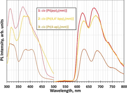
Figure 11 Photoluminescence excitation (left/thinner curves) and emission (right/thicker curves) spectra for solid samples of 1, 2, and 3 at 77 k.

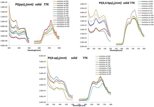
Table 9 Select bond lengths, angles, and torsion angles for Pt(2,2ʹ-bpy)(mnt). Experimental values for Pt(2,2ʹ-bpy)(mnt) taken from ^[4747]

Bond Length (Å)			Angle (°)
	Experimental	Theoretical		Experimental	Theoretical
Pt1—S2	2.243	2.303	S1—Pt1—S2	89.8	89.2
Pt1—S1	2.249	2.303	N5—Pt1—S1	95.8	96.1
Pt1—N5	2.047	2.101	N5—Pt1—S1	175.0	96.1
Pt1—N3	2.035	2.101	N3—Pt1—N5	79.9	78.6
S1—C2	1.734	1.756	C1—S2—Pt1	103.8	103.8
S2—C1	1.730	1.756	C1—C2—S1	121.0	121.6
N1—C3	1.139	1.187	Torsion Angle (°)
C2—C4	1.436	1.450		Experimental	Theoretical
C2—C1	1.367	1.392	PtS2C2—N3 Ring	3.59	0.00
C4—N2	1.136	1.187	PtS2C2—N5 Ring	2.09	0.00
C3—C1	1.431	1.450	N3Ring—N5 Ring	4.51	0.00

Figure 12 SOMO and SOMO-1 for the convergent Pt(2,2ʹ-bpy)(mnt) complex along with experimental oxidation and reduction values (in DMF) taken from ^[50] and calculated oxidation and reduction potentials.

Figure 13 Calculated absorption spectra of Pt(2,2ʹ-bpy)(mnt) with orbital contours for the transition with the highest oscillator strength.

Nesterov, V. N.; Reinheimer, E. W.; Smucker, B. W. (2,2`-Bipyridine)(1,2-Dicyanoethene-1,2-Dithiolato)Platinum(Ii). IUCrData. 2019, 4(x190158). DOI: 10.1107/S2414314619001585.

 Google Scholar