Figures & data
Fig. 1 The PUB initiative has been designed to lead to a greater harmony of scientific activities, and increased prospects for real scientific breakthroughs. Illustration of the elephant as described by blind people reproduced by permission of Jason Hunt (1999, from Sivapalan et al. 2003).
Fig. 2 In the quest for better predictions not only in ungauged basins, one initial objective of PUB was to move away from models strongly based on calibration towards those with a stronger emphasis on increased levels of understanding (from Sivapalan et al. 2003).
Fig. 3 Observed continuous longitudinal and temporal temperature profile of the Maisbich stream in Luxembourg between 24 April and 1 May 2006. Clear temperature jumps can be seen at the location of the groundwater inflows (from Selker et al. Citation2006a, © 2006 John Wiley and Sons).
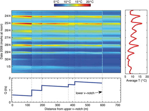
Fig. 4 Based on earlier work by Tromp-van Meerveld and McDonnell (Citation2006a, 2006b), this figure illustrates how local heterogeneities in the subsurface, such as soil pipes, control the hillslope connectivity, and as emergent properties in turn give rise to threshold-like subsurface stormflow response on the small catchment scale (from Troch et al. 2009a, with permission Ciaran Harman, © 2008 Blackwell Publishing Ltd.). It indicates the importance of distinct thresholds controlling emergent behaviour at different scales from the plot to the catchement scale.
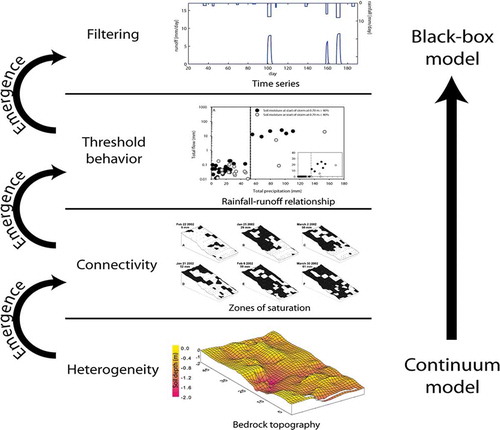
Fig. 5 Performance of a model with respect to streamflow (Fq), groundwater dynamics (Fw) and stream tracer response (Fi). Step-wise model improvements from the least complex SoftModelq (red) to the most complex SoftModeli (yellow) determine the orthogonal trajectory in objective space (from Fenicia et al. Citation2008a, © 2008 John Wiley and Sons).
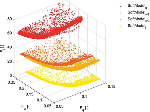
Fig. 6 Three types of information available for constraining a predictive model (from Gupta et al. Citation2008, © 2008 John Wiley and Sons, Ltd.).
Fig. 7 Example of a modelled hydrograph (90% confidence interval) based on calibration using (a) a deterministic rating curve and (b) a rating curve including uncertainty (from McMillan et al. 2010, © 2010 John Wiley and Sons, Ltd.). This result illustrates the effect of rating curve uncertainty, which may add uncertainty to model predicitions, especially for estimating extremes.
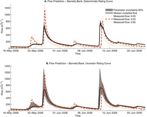
Fig. 8 The 5% and 95% plausibility intervals of output based on posterior parameter distributions with multiple constraints (recession slope, spectral properties, monthly water balance): discharge (top) and evaporation (bottom, from Winsemius et al. 2009, © 2009 John Wiley and Sons, Ltd.). This example illustrates the potential value of applying constraints based on “soft” data and emergent properties, to reduce predictive uncertainty especially for predictions in data-scarce regions.
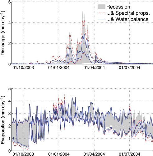
Fig. 9 Spatial patterns of selected calibrated model parameters—top: maximum soil moisture storage FC (mm); centre: potential evaporation limit LP (mm); and bottom: nonlinearity parameter β (-)—for the calibration periods 1987–1997 (left) and 1976–1986 (right) (from Merz and Blöschl 2004, © 2004 Elsevier). This illustrates the potential of using spatial proximity as a proxy for functional proximity in densely gauged regions.
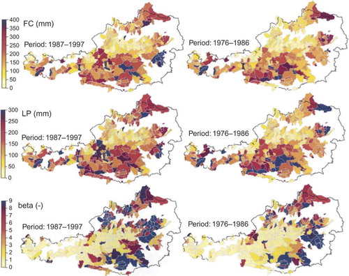
Fig. 10 Based on analysis of flow duration and regime curves, and the inferred influence of temperature, aridity, seasonality and phenology, the circled areas represent regions of process similarity. This indicates the need for models that represent the same dominant processes for catchments within the circled regions (from Ye et al. 2012)—an example of how careful synthesis of catchment emergent properties and signatures can guide the model design and selection process for data-scarce regions in particular.
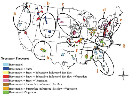
Fig. 11 Modelled (black) and observed (grey) daily (a) evapotranspiration rates (ET) and (b) net CO2 assimilation rates (Ag,tot). The means of the observed and modelled time series are given, together with the mean absolute errors (MAE) and Pearson’s r values, indicating the goodness of fit (from Schymanski et al. 2009, © 2009 John Wiley and Sons, Ltd.).
Fig. 12 Outline of how scientific understanding evolved and the way of thinking shifted towards new questions during the PUB Decade.
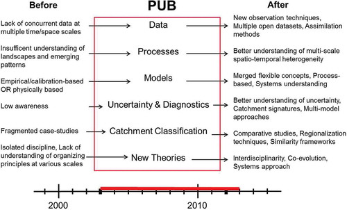
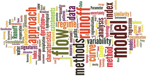
Fig. 13 Word cloud summarizing the relevant aspects and concepts of hydrology throughout the PUB Decade, based on the index of Böschl et al. (2013).