Figures & data
Fig. 1 Results of the simulation studies (see Section 6): (a) exemplary time series simulated using the procedure and parameters outlined; (b) convergence of the estimators for the variance equation (16): solid lines indicate ±2 SE range from equation (22); (c) convergence of the variance of the estimated variance: the markers indicate the sample variance obtained by running 50 simulations for each N; solid lines are from equation (20); (d) convergence of the estimators for the variance equation (16); solid lines indicate the ±2 SE range from equation (21); (e) convergence of the variance of the estimated variance: the markers indicate the sample variance obtained by running 50 simulations for each N; solid lines are from equation (21); and (f) comparison of the empirical normalization factor of equation (36) with the number of samples N; solid lines are from equation (36).
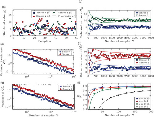
Fig. 2 Results of case study 1: calibration constants, RMS errors (square root of estimated variance) and autocorrelations. The window sizes wc and we are expressed in months: (a) the soil moisture time series; (b) estimated α for ASCAT; (c) estimated β for ASCAT; (d) estimated RMS of ASCAT, wc = we; (e) estimated RMS of ASCAT wc we; (f) estimated RMS of ASCAT, in ASCAT climatology, wc = we; (g) estimated RMS of ASCAT, in ASCAT climatology, wc we; (h) autocorrelation of ASCAT errors, τ = 1 d; (i) autocorrelation of ASCAT errors, τ = 10 d, wc = we; and (j) autocorrelation of ASCAT errors, τ = 10 d, wc we.
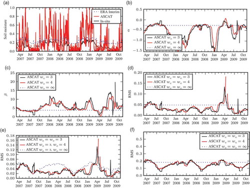
Fig. 2 (Continued)
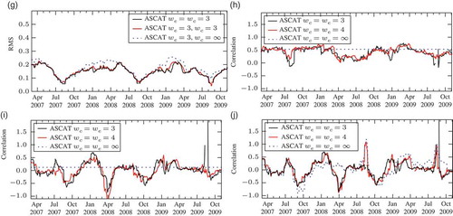
Table 1 Overview of the soil moisture probes
Fig. 3 Soil moisture measured by the five sensors at Station 115 of the UDC_SMOS network.
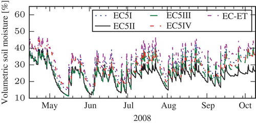
Table 2 Estimated variances
Table 3 Estimated covariances
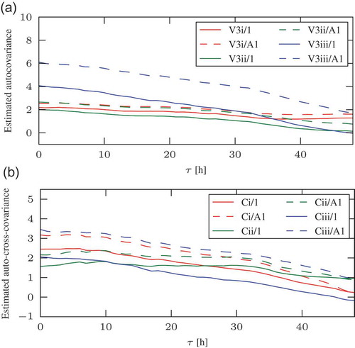
Fig. 4 Different estimates of (a) the autocovariance and (b) the auto-cross-covariance function of sensor EC-ET. The legend refers to the combination and the period during which α is estimated, e.g. V3i/A1 denotes the estimate with combination V3i, where α was determined during period A1.