1,075
Views
19
CrossRef citations to date
0
Altmetric
Special issue: Weather Radar and Hydrology

Forecasting flash floods using data-based mechanistic models and NORA radar rainfall forecasts

Prévision des crues éclair à l’aide de modèles mécanistes fondés sur les données et prévisions pluviométriques du système radar NORA

, &
Pages 1403-1417 | Received 08 Nov 2013, Accepted 17 Jul 2013, Published online: 23 Jan 2014

Figures & data

Table 1 Occurrence of NORA events summarized by year and month. Zero values are left blank

Fig. 1 Summary of the performance of the hourly accumulated NORA precipitation forecasts against those generated by persistence and COSMO2 at lead-times of up to 6 h. For a definition of the verification scores presented, see Wilks (Citation1995) and Panziera et al. (Citation2011). Lead-time is given as the start of the accumulation period.
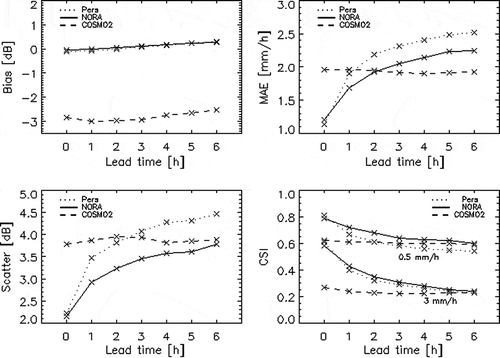
Fig. 1 Summary of the performance of the hourly accumulated NORA precipitation forecasts against those generated by persistence and COSMO2 at lead-times of up to 6 h. For a definition of the verification scores presented, see Wilks (Citation1995) and Panziera et al. (Citation2011). Lead-time is given as the start of the accumulation period.

Fig. 2 One year of calibration data showing the observed data (•) and simulated DBM output (––––).

Fig. 2 One year of calibration data showing the observed data (•) and simulated DBM output (––––).

Table 2 Summary statistics of forecasting performance during calibration of the DBM model using data assimilation with the assumption that future rainfall is known. Values in parentheses represent the statistics computed only when discharge >75 m3/s. Results for the model run without data assimilation are shown for comparison

Table 3 Summary statistics of forecasting performance during validation of the DBM using data assimilation with the assumption that future rainfall is known. Values in parentheses represent the statistics computed only when discharge >75 m3/s

Fig. 3 Calibration forecast (made using observed rainfall) for a large event in the autumn of 1993. Observed data (•) and forecasts using data assimilation at lead-times of 1 h (–––), 3 h (......) and 5 h (- - - -) are shown together with the model output using no data assimilation (- . - . -).
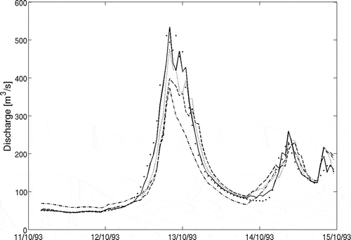
Fig. 3 Calibration forecast (made using observed rainfall) for a large event in the autumn of 1993. Observed data (•) and forecasts using data assimilation at lead-times of 1 h (–––), 3 h (......) and 5 h (- - - -) are shown together with the model output using no data assimilation (- . - . -).

Table 4 Summary statistics of forecasting performance using predicted precipitation during time periods where NORA forecasts are available. Data for the first 2 h lead-time where NORA forecasts are not used are shown for completeness. Performance when it is assumed the observed rainfalls are known is shown in parentheses

Fig. 4 Scatter plots of the observed discharge vs that forecast with lead-times of (a) and (b) 1 h; and (c) and (d) 2 h. For each lead-time, the dataset is separated into forced (left-hand panes) and unforced (right-hand panes) time- steps to show the difference in distribution.
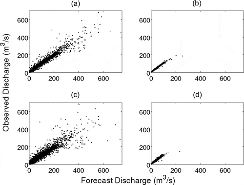
Fig. 4 Scatter plots of the observed discharge vs that forecast with lead-times of (a) and (b) 1 h; and (c) and (d) 2 h. For each lead-time, the dataset is separated into forced (left-hand panes) and unforced (right-hand panes) time- steps to show the difference in distribution.

Fig. 7 Forecasts for lead times of up 6 h issued for the largest of the validation events in 2009. The shaded area represents the 95% prediction interval, solid lines the deterministic model forecast and points the observed discharge.
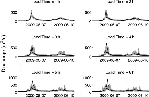
Fig. 7 Forecasts for lead times of up 6 h issued for the largest of the validation events in 2009. The shaded area represents the 95% prediction interval, solid lines the deterministic model forecast and points the observed discharge.

Fig. 5 Scatter plots of against used in the estimation of non-parametric error distribution which is represented by the 95% prediction interval (shaded area) for various forecast lead-times.
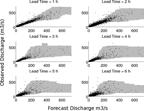
Fig. 5 Scatter plots of against used in the estimation of non-parametric error distribution which is represented by the 95% prediction interval (shaded area) for various forecast lead-times.
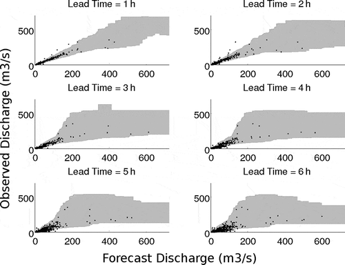
Fig. 6 Scatter plots of against for the validation storms in 2009 overlaying the non-parametric error distribution which is represented by the 95% prediction interval (shaded area) for various forecast lead-times.
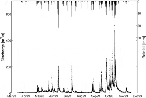
Fig. 6 Scatter plots of against for the validation storms in 2009 overlaying the non-parametric error distribution which is represented by the 95% prediction interval (shaded area) for various forecast lead-times.

Reprints and Corporate Permissions

Please note: Selecting permissions does not provide access to the full text of the article, please see our help page How do I view content?

To request a reprint or corporate permissions for this article, please click on the relevant link below:

Academic Permissions

Please note: Selecting permissions does not provide access to the full text of the article, please see our help page How do I view content?

Obtain permissions instantly via Rightslink by clicking on the button below:

If you are unable to obtain permissions via Rightslink, please complete and submit this Permissions form. For more information, please visit our Permissions help page.