On a PUB methodology from Chinese lessons

Figures & data

Fig. 1 The relationships among the possible solutions that a clever housewife may find when she wants to feed her hungry family but has no rice, including Borrowing (B) from neighbours or shops, using substitutes from within the home (S1), using substitutes from outside the home (S2), using substitutes (S3) such as new food products, and Generating (G) by planting rice seed immediately. The forcing factors in the figure are those driving or helping the housewife to find substitutes, such as the location of the places where she can find food, time to get there, the family’s favorite food, road conditions, etc.

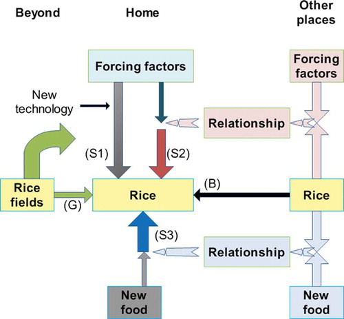
Fig. 2 With reference to PUB, the relationship among Borrowing (B), using substitutes from within the ungauged basin (S1), using substitutes from gauged basins by grouping them into n groups with similar scaled hydrological elements (HE), scaled by the scale variable V (S2-1), using proxy data as substitutes (S3) and Generating (G).

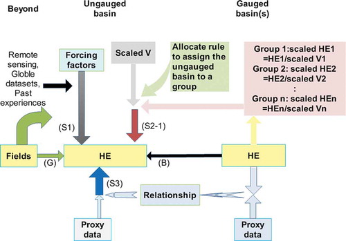
Fig. 3 The same as Fig. 2, but with the the parts for S2-1 in Fig. 2 replaced with the parts for S2-2.

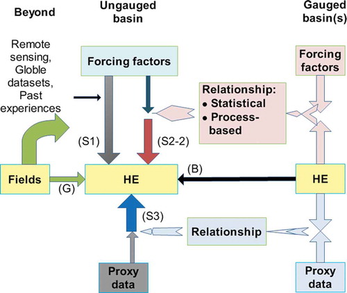
Table 1 The relationship between TFT proposed in Blöschl et al. (2013) and BSG proposed in this paper.

BSG	TFT	Features
Borrowing	Geostatistical methods Estimation from short runoff records	Borrowing HE from gauged catchment(s)
Substituting: S1	(Fully process-based, analytical, or simplified with the aim of no calibration) Continuous rainfall–runoff models Estimation from short runoff records	Using substitutes (The fully process-based model; routine data of climate and catchment feature) mostly from the ungauged basin
Substituting: S2-1	Index method Derived distribution method Estimation from short runoff records	Using substitutes (the scaled hydrological signature from similar gauged basins and the routine data for scaling in ungauged basin)
Substituting: S2-2	Regression method (Other process-based) Continuous rainfall–runoff models Estimation from short runoff records	Using substitutes (the other process-based model, regression model from similar and dissimilar gauged basins and the routine data from ungauged basin)
Substituting: S3	Methods that exploit proxy data Estimation from short runoff records	Using substitutes (statistical relationship between special data and HE from gauged basins; special data from ungauge basin)
Generating	–	Obtaining and accumulating HE by doing field and indoor experiments

Note: Routine data include climate (aridity index, annual precipitation, etc.) and catchment features (vegetation index, landscape index, soil index, river top-width, etc.). Special data include tree ring, polar motion, etc.

Fig. 4 Distribution of the methods used in the work of 20 case studies in Blöschl et al. (2013) according to BSG.

Fig. 5 Years of the earliest publications using each of the BSG methods to predict the hydrological signatures: annual runoff (A), seasonal runoff (S), low flow (L), floods (F), flow duration curve (FDC) and hydrograph (H).

Fig. 6 The distribution of the number of the references cited by Blöschl et al. (2013) according to the different hydrological signatures and BSG framework. From top to bottom along the vertical y-axis the order is annual runoff, seasonal runoff, low flows, floods, flow duration curves and runoff hydrograph. From left to right along the horizontal x-axis the order is B, S1, S2-1, S2-2, S3 and G. The left panel is before the PUB decade and the right panel is during/after the PUB decade. The upper and lower panels present the same results but displayed differently.

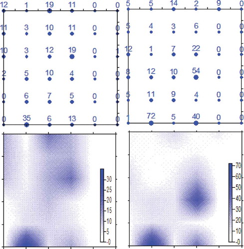
Fig. 7 (a) The controlled area per station (km²) in China and other places in the world. (b) The station network density of each sub-catchment of the Yellow River Basin, the second longest river in China; the x-axis displays the location from Western China to East China (Liu et al. 2010).

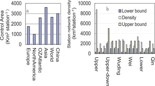
Table 2 The number of articles in the literature focusing on PUB in China categorized with the BSG framework.

	B	S1	S2-1	S2-2	S3	G
Before 2002	4	2	0	11	1	2
After 2002	12	51	2	33	5	5

Blöschl, G., et al., eds., 2013. Runoff prediction in ungauged basins: synthesis across processes, places and scales. Cambridge: Cambridge University Press.

 Google Scholar

Liu, S., Liu, C., and Zhao, W., 2010. Towards the methodology for Predictions in Ungauged Basins. Progress in Geography, 29 (11), 1333–1339. (In Chinese with English Abstract.)

 Google Scholar