Figures & data
Fig. 1 SWIM structure.
Table 1 Overview of the most important applications of SWIM.
Table 2 List of major parameters used for hydrological calibration of SWIM.
Table 3 Nash-Sutcliffe (Nash and Sutcliffe Citation1970) efficiency (NSE) and logarithmic Nash-Sutcliffe efficiency (LNSE) for the calibration and validation periods for the selected gauges (see full version in Huang et al. Citation2013b).
Fig. 2 Simulated and observed water discharge (left) at the gauges (a) Intschede (Weser) and (b) Hofkirchen (Danube) in the calibration period 1986–1989, and the corresponding average daily discharge (right) for the same stations in the same period (see an extended version in Huang et al. Citation2010). The corresponding NSE values for (a) and (b) are 0.92 and 0.90, respectively.
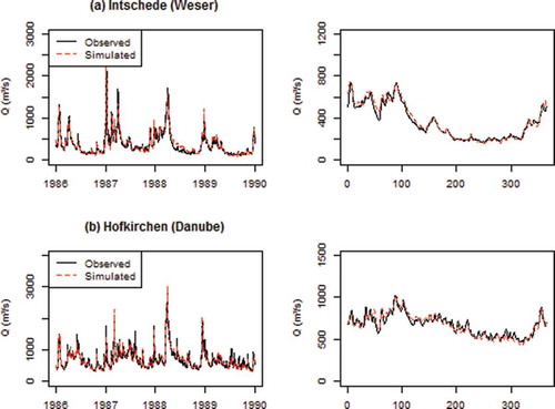
Fig. 3 Comparison of the simulated 50-year flood and low-flow levels at 29 gauges in Germany with the observed ones for the period 1961–2000.
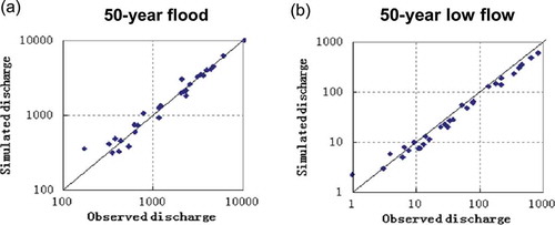
Fig. 4 Generalized extreme value (GEV) plots for the annual maxima of observed daily discharge and simulated discharge using observed climate data of 1961–2000 for four selected gauges in Germany; their drainage areas are indicated in .
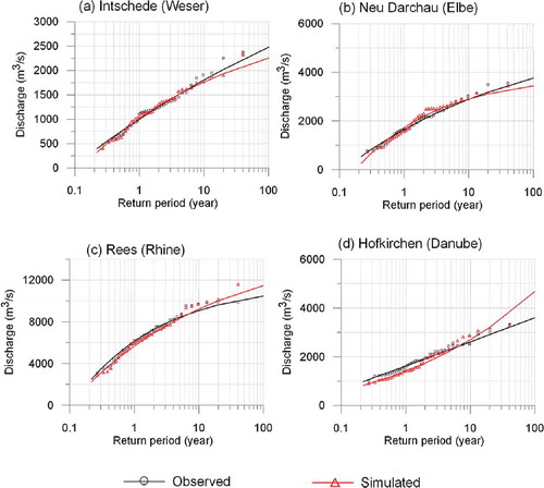
Fig. 5 Return level plots for the observed and simulated annual minimum 7-day discharge (AM7) at four selected gauges in Germany in the period 1961–2000; their drainage areas are indicated in .
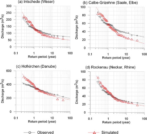
Fig. 6 Example of validation for sediment load dynamics: daily dynamics of simulated (negative values from the top of the diagram) and measured sediment load (positive values) in the Glonn catchment (Germany) for six years in the period 1981–1990 (see more examples in Krysanova et al. Citation2002).
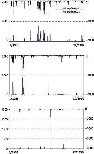
Fig. 7 Water quality modelling with SWIM in the Saale River catchment, gauge Groß Rosenburg (Germany): comparison of measured and simulated mean monthly average values with standard deviations for nitrate nitrogen (NO3-N), phosphate phosphorus (PO4-P), ammonium nitrogen (NH4-N), and chlorophyll a concentrations for the period 1996–2003.
Fig. 8 Comparison of observed and modelled groundwater table for three observation wells in the Nuthe catchment (see an extended version in Hattermann et al. Citation2006).
Fig. 9 (a) Spatial patterns of NO3-N uptake by plants in wetlands and riparian zones; and (b) comparison of NO3-N concentrations with (Nrip+) and without (Nrip-) considering retention in wetlands and riparian zones in the Nuthe catchment as a long-term average daily dynamics in 1993–1998 (see daily dynamics in Hattermann et al. Citation2006).
Fig. 10 Comparison of average measured (according to statistical data) and simulated yield of winter wheat for the German part of the Elbe basin (Germany) in 1996–1999.
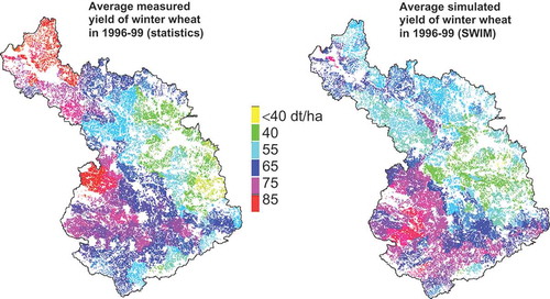
Fig. 11 Simulated and observed snow depth (left) at two selected climate stations for the period 1981–1990 and the corresponding average daily snow depth (right) for the same stations in the validation period (1961–1980).
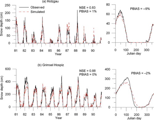
Fig. 12 Reservoir module performance during the dry period with and without reservoir management for the Niger basin, gauge Koulikoro (121 000 km2).
Fig. 13 Water discharge simulation with and without inundation module, average year representing both the calibration and validation periods.
Fig. 14 Seasonal water discharge in the scenario periods (2031–2060) including 80 (dark grey) and 100 (light grey) realizations and the median of 100 realizations (black line) compared to the simulated discharge for the reference period 1961–1990 for six basins: (a) the Ems (gauge Versen); (b) the Weser (gauge Intschede); (c) the Saale (gauge Calbe-Grizehne); (d) the Danube (gauge Hofkirchen); (e) the Main (gauge Frankfurt-Osthafen); and (f) the Neckar basin (gauge Rockenau SKA).
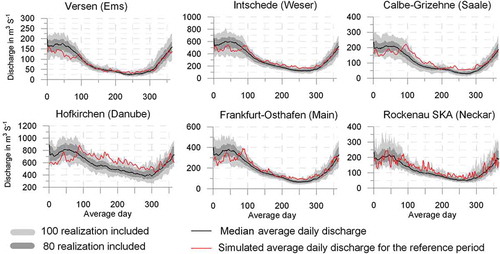
Fig. 15 Median return period for the 50-year low flow (averaged from those driven by REMO, CCLM and Wettreg scenarios) with the change directions agreed by 6–10 projections for the periods (a) 2021–2060 and (b) 2061–2100.
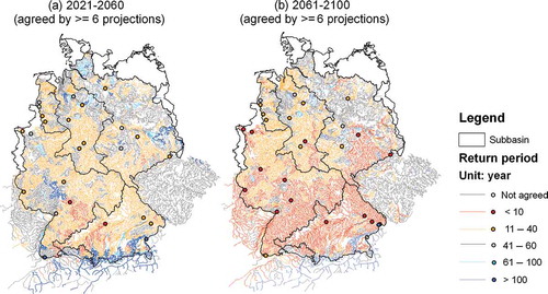
Fig. 16 Left: extreme value functions (GPD) fitting the observed and simulated daily flows at gauge Archleiten (Danube) in the period 1951–2000; right: comparison of flood damages at river section Archleiten in 1961–2000 calculated using runoff simulated by SWIM (sim) and observed runoff (obs) and applying damage functions provided by the German Insurance Association (GDV).
Fig. 17 Relative changes in flood related damages as average values of seven scenario runs in 2041–2070 compared to the average damages in 1961–2000 (defined as 100%). For further explanations see Hattermann et al. (Citation2014).
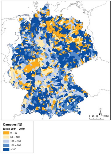
Table 4 Description of the land-use and management change scenarios simulated with SWIM in two different sub-catchments of the Elbe basin in Germany (reference periods for the Rhin basin: 2001–2005, for the Saale basin: 1996–2003).
Fig. 18 Percentage change of selected mean SWIM model outputs under land-use change scenario conditions compared to the reference conditions in two different catchments within the Elbe River basin (for detailed description of the single scenario conditions see ). The size of circle represents the increase (black) and decrease (white) in percent scaled to 100.
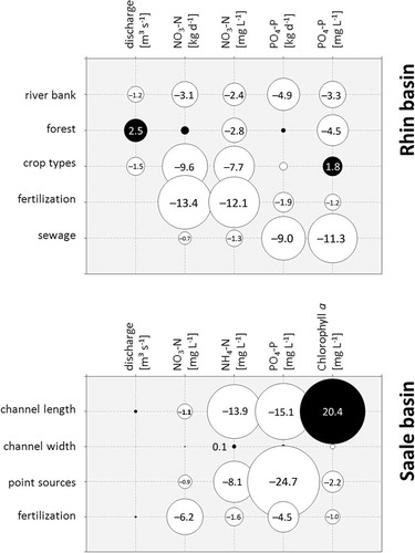
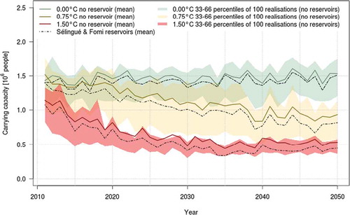
Table 5 Wetland capacity for rice production to support people (units: number of people in million) in the IND for the period 2041–2050.
Fig. 19 Simulated carrying capacity of rice production in the Inner Niger Delta. Continuous coloured lines represent the means of 100 realizations for the three scenarios without upstream reservoirs. Dashed lines represent the means of 100 realizations with two upstream reservoirs included in simulations. The coloured bands represent 33–66 percentiles of 100 realizations.