
Figures & data
Figure 1. Daily water consumption time series for Mashhad between March 2009 and July 2013. The time series includes a wide range of values from 270 000 to 830 000 m3 over a year. Dashed line shows the linear trend of demand time series. Ovals show some extreme effects of the coincidence of the two calendars that result in jumps (each represents a special religious holiday) in daily water consumption.
Figure 2. Load duration curve of Mashhad daily water consumption showing the approximate frequency of each value in the time series. The proportion of each class is inserted in the legend.
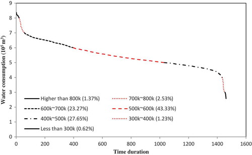
Figure 3. Schematic architecture of a feedforward multilayer perceptron with one hidden layer. A sigmoid activation function is used for the hidden layers and a linear activation function is assigned to the output node.
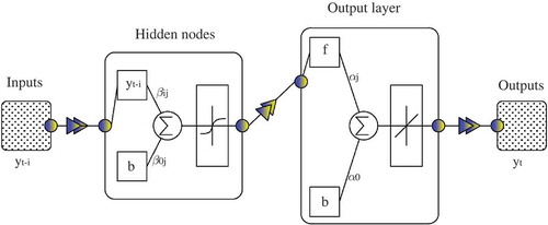
Figure 4. Schematic architecture of a cascade-forward network with one hidden layer. A sigmoid activation function for the hidden layers and a linear activation function for the output node are desired for forecasting problems.
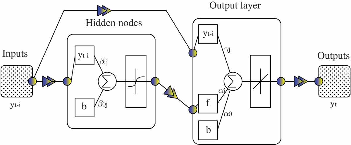
Figure 5. Schematic architecture of a typical radial basis network which has only two layers.
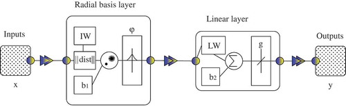
Table 1. Ten categories of input data to neural networks. Among these variables, ,
,
,
,
and
are the calendar-based inputs, which are used to consider effects of population fluctuations.
Table 2. Values of the performance indices calculated using the validation dataset for 14 forecasting lead times. For each lead time, the performances of the three types of neural networks are presented, with the best in bold.
Figure 6. (Top) Regression coefficient, R and MSE of validation dataset vs goal parameter. (Bottom) Regression coefficient and MSE of validation dataset vs spread parameter. and
provide the best performance.
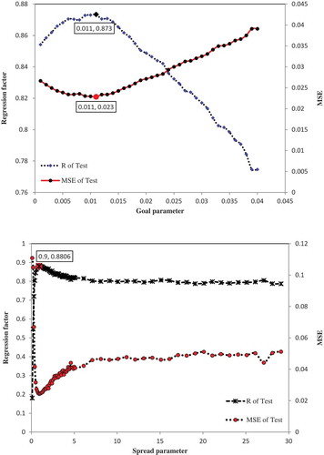
Figure 7. The best and the worst validation results of the selected radial basis networks using the test dataset. Validation of test data for (a) 5-day ahead forecasting with R = 0.9178 and MSE = 0.0172, (b) 10-day ahead forecasting with R = 0.8556 and MSE = 0.0255, (c) 13-day ahead forecasting with R = 0.8636 and MSE = 0.0273, (d) 14-day ahead forecasting with R = 0.9167 and MSE = 0.0158. The vertical axis is the normalized range of water consumption values. Among 14 radial basis networks, models 5 and 14 (which forecast the 5th and 14th day ahead) provide the maximum value of R and minimum value of MSE respectively, models 10 and 13 (which forecast the 10th and 13th day ahead) provide the minimum value of R and maximum value of MSE respectively.
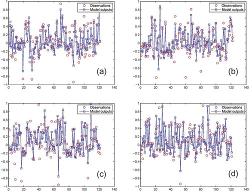
Figure 8. The actual time series vs the forecasts of the selected radial basis network trained with/without calendar-based inputs. Forecasts from 100 runs of the radial basis network are exactly the same.
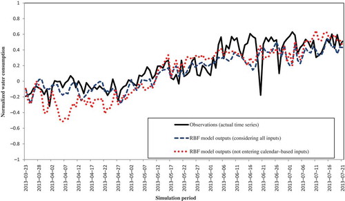
Table 3. Overall results of the three types of neural networks.
Figure A1. The actual time series vs the forecast offset resulting from 100 multilayer perceptron model runs. + signs represent forecasts of the model trained with all inputs and the dashed line connects their mean values in each forward lead time. Dots (red) represent forecasts of the model trained excluding calendar-based inputs and the dotted (red) line connects their mean values in each forward lead time.
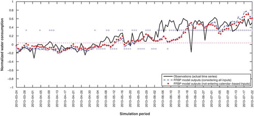
Figure A2. The actual time series vs the forecast offset resulting from 100 one-hidden-layer cascade-forward model runs. Symbols as in Fig. A1.
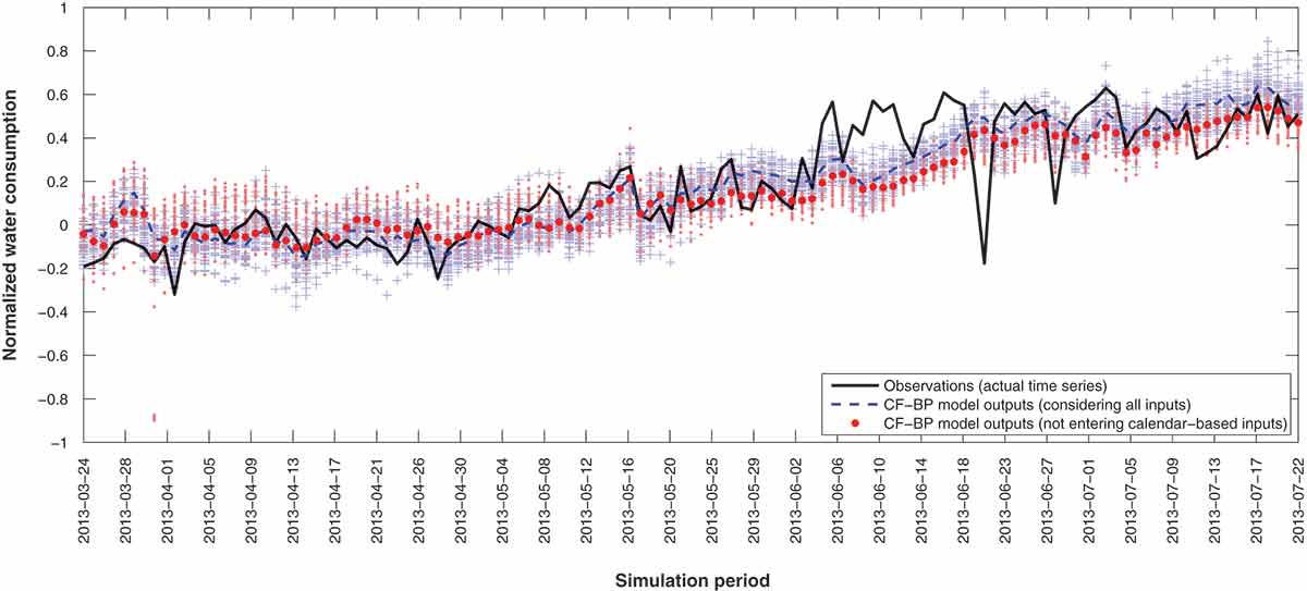
Figure A3. The actual time series vs the forecast offset resulting from 100 four-hidden-layer cascade-forward model runs. Symbols as in Fig. A1.
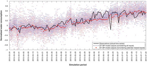
Table A1. Overall results of all repetitions for multilayer perceptron and radial basis function models.
Table A2. Overall results of all repetitions for one-hidden-layer and four-hidden-layer cascade-forward networks.