Figures & data
Figure 1. Comparison of the outflow hydrographs of the Lag-and-Route and Kalinin-Miljukov models and of the inflow hydrographs of the reverse Lag-and-Route and Reservoirs-in-Series models: top panel qin = Q*sinωt and bottom panel qin = Q*(1 – cosωt)/2; the outflows of the single-reach Muskingum model demonstrate that model’s shortcomings (however, the slope break in the top panel’s hydrograph disappears for the smoother inflow function (1 – cosωt)/2 (bottom panel)).
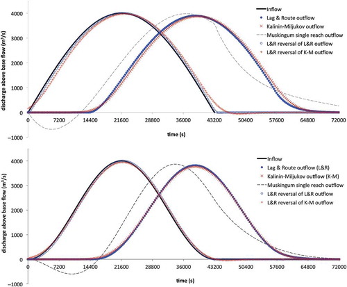
Figure 2. Reverse routing FD scheme and low-pass filtering—symmetric second-order 11-point filter.
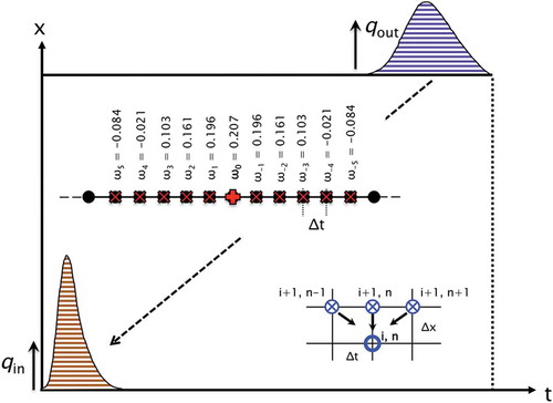
Figure 3. Lag-and-route reverse routing of error-seeded outflow data with filtering (for filter applied only on the outflow data, see inset) and without filtering.
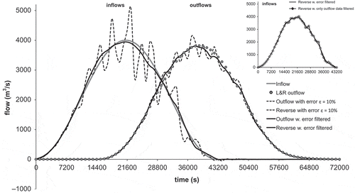
Figure 4. Concept of reservoir control with example: controlled reservoir outflows (discharges above baseflow) calculated by the reservoirs-in-series model from filtered (solid line with non-filled circles), and unfiltered (grey solid line) data and by the lag-and-route model (solid line with solid circles) from unfiltered data.
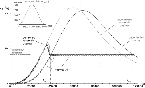
Figure 5. Pollutographs (C): observed (black dots) Cin and breakthrough curves, and lag-and-routed forward (L&R) (+) and reverse recovered (empty circles) curves.
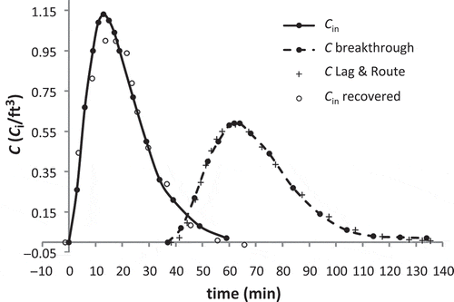
Table 1. Concentrations calculated forward and reverse with the lag-and-route model.
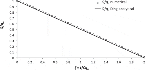
Figure A1. Comparison of numerical quasi-nonlinear solution to Ding’s analytical solution.