Assessment of radar-based locally varying anisotropy on daily rainfall interpolation

Figures & data

Figure 1. Location of (a) the study area in Queensland, Australia, and (b) the 117 daily gauge stations (black dots) within the range of the Mt. Stapylton weather radar station (near Brisbane) (red dot); the radar image in log10(mm) scale is for 28-03-2014.

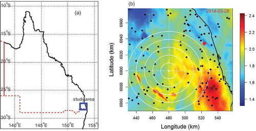
Table 1. Basic properties of selected wet days.

Date	Number of gauges	Wetted area ratio			Average wet gauge amount (mm)			Maximum wet gauge amount (mm)			Gauge–collocated correlation
		Gauge	Collocated	Radar	Gauge	Collocated	Radar	Gauge	Collocated	Radar
14 January 2014	109	0.450	0.248	0.191	3.2	2.5	2.3	7.4	6.7	11.1	0.57
20 February 2014	109	0.184	0.184	0.166	15.0	6.0	5.9	31.4	15.2	23.5	0.92
24 February 2014	102	0.578	0.402	0.311	4.4	4.5	4.2	15.0	18.4	21.6	0.70
25 February 2014	111	0.568	0.297	0.240	4.8	3.9	3.9	17.4	11.4	19.5	0.66
05 March 2014	109	0.560	0.367	0.284	6.9	4.6	6.4	24.2	17.2	45.4	0.78
09 March 2014	104	0.356	0.481	0.439	2.9	3.5	3.0	6.6	10.9	16.6	0.62
10 March 2014	98	0.786	0.510	0.391	5.7	3.6	3.5	22.1	13.2	17.6	0.63
25 March 2014	107	0.935	1.000	0.996	19.5	22.8	24.5	110.2	82.3	168.3	0.79
26 March 2014	107	0.991	1.000	1.000	24.1	24.4	21.7	58.0	59.8	99.2	0.72
27 March 2014	108	0.954	1.000	1.000	11.3	37.0	36.8	37.2	130.3	160.8	0.21
28 March 2014	109	1.000	1.000	1.000	133.9	87.1	77.6	319.4	233.6	266.5	0.83
14 April 2014	94	0.830	0.436	0.512	6.6	3.7	3.5	30.2	22.0	27.4	0.65

Figure 2. (a) Radar data empirical correlogram and (b) correlogram of the gauged data for 28-03-2014. Concentric circles encompass areas within {10, 20, 30, 40, 50} km radius from the correlogram map centre.

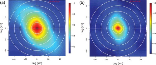
Figure 3. Correlograms generated by the regional options (0–3) parameter sets with contours superimposed; radar data of 05-03-2014.

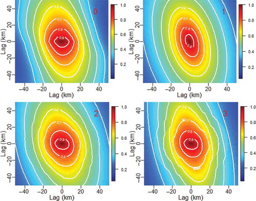
Figure 4. Variation of the anisotropy ratio with the lag distance of the regional options parameter sets using radar data.

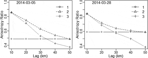
Table 2. Estimated correlogram parameters defined in equation (4) of the regional option 1 using gauge and radar data. L_u: major axis correlation length; η: anisotropy ratio; θ: anisotropy direction; a_n: correlogram sill.

Date	Lu (km)		η		θ (degrees)		an
	Gauge	Radar	Gauge	Radar	Gauge	Radar	Gauge	Radar
14 January 2014	22.1	35.6	0.78	0.60	5	122	0.87	1.00
20 February 2014	22.6	66.3	0.88	0.42	80	130	0.90	1.00
24 February 2014	22.4	104.3	0.81	0.42	99	97	0.91	1.00
25 February 2014	21.6	61.4	0.81	0.60	0	96	0.89	1.00
05 March 2014	23.8	84.2	0.91	0.49	93	103	0.90	1.00
09 March 2014	9.7	39.9	0.83	0.82	108	141	0.97	0.99
10 March 2014	18.4	54.2	0.86	0.59	84	97	0.94	1.00
25 March 2014	18.7	30.3	0.91	0.79	90	113	0.90	1.00
26 March 2014	17.6	20.4	0.67	0.89	99	93	0.94	1.00
27 March 2014	19.7	60.2	0.88	0.77	133	70	0.92	1.00
28 March 2014	19.4	40.9	0.65	0.59	106	121	0.95	1.00
14 April 2014	28.1	40.0	0.63	0.84	4	11	0.88	1.00

Figure 5. Locally varying anisotropy (LVA) direction (θ, left panels) and the major axis correlation length (L_u in km, right panels), for radii of (a) 10 km, (b) 30 km and (c) 50 km.

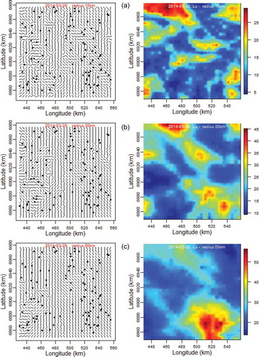
Table 3. Estimated performance statistics using the different correlograms for two wet days, 10-fold case. RMSE: root mean square error; MB: mean bias; MAB: mean absolute bias; MIQR: mean inter quartile range; SD: mean standard deviation in the Gaussian domain.

Correlogram option	24/02/2014					28/03/2014
	RMSE	MB	MAB	MIQR	Mean SD	RMSE	MB	MAB	MIQR	Mean SD
Gauge
G_REG_0	1.74	−0.35	1.05	2.27	0.66	37.03	−4.42	21.5	47.4	0.68
G_REG_1	1.69	−0.28 −0.32	1.06	2.32	0.66	37.31	−4.05	21.4	46.9	0.68
G_REG_2	1.70		1.04	2.31	0.66	37.38	−4.05	21.4	46.9	0.68
G_REG_3	2.04	−0.60	1.29	2.66	0.78	36.46	−3.78	20.8	46.7	0.67
Radar
R_REG_0	1.96	−0.13	1.21	1.05	0.29	38.42	−3.34	21.4	29.6	0.43
R_REG_1	1.94	−0.04	1.21	1.12	0.32	38.19	−3.31	21.8	32.1	0.47
R_REG_2	1.85	−0.08	1.16	1.13	0.32	38.30	−3.23	21.8	32.2	0.47
R_REG_3	1.77	−0.11	1.12	1.11	0.31	38.44	−3.81	21.9	34.2	0.52
LVA
R_LVA_0	1.69	−0.25	1.11	2.39	0.77	37.05	−3.92	20.9	43.9	0.63
R_LVA_1	1.88	−0.49	1.16	2.90	0.88	38.29	−4.26	22.6	53.0	0.76
R_LVA_2	1.76	−0.38	1.11	2.71	0.84	37.07	−3.64	21.5	49.4	0.70
R_LVA_3	1.74	−0.28	1.14	2.44	0.78	37.18	−3.81	21.1	45.1	0.65
R_LVA_4	1.71	−0.19	1.11	2.26	0.74	37.87	−3.78	21.3	41.9	0.61
R_LVA_5	1.80	−0.22	1.17	2.03	0.70	38.09	−4.07	21.6	39.9	0.58

Table 4. Ranked performance statistics for the correlograms, where 1 denotes best and 14 worst: 10-fold case for 24 February 2014. RMSE: root mean square error; MB: mean bias; MAB: mean absolute bias; MIQR: mean inter quartile range; SD: standard deviation in the Gaussian domain; correlogram option prefix G for gauged and R for radar.

Correlogram option	RMSE	MB	MAB	MIQR	Mean SD
G_REG_0	5	4	2	7	5
G_REG_1	2	6	3	9	5
G_REG_2	3	5	1	8	7
G_REG_3	14	1	14	12	11
R_REG_0	13	11	13	1	1
R_REG_1	12	14	12	3	4
R_REG_2	10	13	10	4	3
R_REG_3	8	12	7	2	2
R_LVA_0	1	8	5	10	10
R_LVA_1	11	2	9	14	14
R_LVA_2	7	3	4	13	13
R_LVA_3	5	7	8	11	12
R_LVA_4	4	10	6	6	9
R_LVA_5	9	9	11	5	8

Table 5. Ranked performance statistics for the correlograms (1 for best and 14 for worst): 10-fold case over all 12 wet days. See Table 4 for abbreviations.

Correlogram option	RMSE	MB	MAB	MIQR	Mean SD
G_REG_0	1	8	1	7	6
G_REG_1	3	4	4	9	8
G_REG_2	2	6	3	8	5
G_REG_3	9	2	14	12	11
R_REG_0	13	14	13	1	1
R_REG_1	14	13	11	3	3
R_REG_2	11	12	10	2	2
R_REG_3	10	11	7	4	4
R_LVA_0	5	7	4	10	10
R_LVA_1	12	1	12	14	14
R_LVA_2	8	3	9	13	13
R_LVA_3	6	5	8	11	12
R_LVA_4	7	9	6	6	9
R_LVA_5	4	10	2	5	7

Figure 6. Comparison of the cross-validation median estimates (solid [blue] line) and the observed values (open circles) for correlogram option R_REG_1. The (red) dotted lines represent the 90% prediction limits. Gauge numbers are in increasing order of the median prediction for easy visualisation.

Table 6. Ranked performance statistics for the correlograms (1 for best and 14 for worst): 10-fold case over all 12 wet days and by conditional simulation. See Table 4 for abbreviations.

Correlogram Option	RMSE	MB	MAB	MITQR	Mean SD
G_REG_0	1	1	1	10	9
G_REG_1	2	3	3	6	6
G_REG_2	3	8	5	8	5
G_REG_3	5	1	10	9	8
R_REG_0	12	14	8	1	1
R_REG_1	14	13	7	4	4
R_REG_2	10	12	4	2	2
R_REG_3	8	11	2	3	3
R_LVA_0	7	7	11	13	13
R_LVA_1	13	3	14	14	14
R_LVA_2	11	5	13	12	12
R_LVA_3	9	6	12	11	11
R_LVA_4	5	9	9	7	10
R_LVA_5	4	10	6	5	7

Figure 7. Comparison of the cross-validation median estimates (solid [blue] line) and the observed values (open circles) for correlogram option R_REG_1 by conditional simulation. See Fig. 6 for explanation.