Figures & data
Figure 1. Location maps and topographic features of the study area, the Toyohira River alluvial fan. The black lines across the river indicate the distance in kilometres, denoted as KP throughout the text. Gauging stations R1 and R2 are located on the river at KP 17.8 and KP 11, respectively. Sky blue, yellow, brown, purple, and green denote topographic features: the low land, Holocene fan, Pleistocene fan, volcanic ash hills, and mountains, respectively.
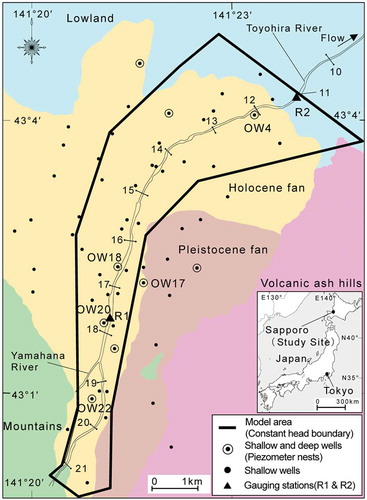
Figure 2. Geological cross-section of the fan subsurface. Inverted open triangles denote piezometric heads in the drought period for analysis. Colours except dark blue (deeper fine deposits in Layer 4) correspond to those in . Profiles of the common logarithm of K at OW18 and 20 are obtained from an undisturbed core analysis in Sakata and Ikeda (Citation2013b).
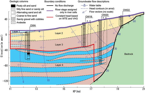
Figure 3. Longitudinal distribution of the median grain size of the bed material in each kilometre (KP) along the Toyohira River.
Figure 4. Observed variations in water levels at gauging stations and observations wells. The locations of gauging stations and monitoring wells are shown in .
Figure 5. Contour maps of (a) WTE and (b) VHG during a drought period for analysis. The monitoring wells correspond with those in . WTE contours are illustrated per 5 m a.m.s.l. Negative (positive) values of VHG indicate downward (upward) hydraulic gradients (dimensionless).
Figure 6. Numerical groundwater flow model in the Toyohira River alluvial fan.
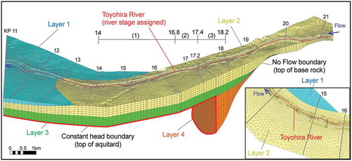
Table 1. Summary of aquifer characteristics and input properties.
Figure 7. Longitudinal distributions of hydraulic conductivity at different depths Z per 10 m with layer numbers (layers 2–4).
Figure 8. Relations between simulated heads Hcal and observed heads Hobs at 43 monitoring wells using (a) the initial model and (b) the optimized model.
Figure 9. Simulated results of (a) specific water loss and (b) surface water budget. Negative and positive values indicate water loss and gain, respectively. Open circles in (b) are average values from previous synoptic discharge survey results.
Table 2. Calculated groundwater fluxes (in and out; m3/s) in the numerical model.
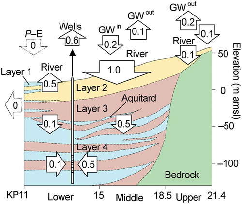
Figure 10. Schematic subsurface groundwater budgets in the Toyohira River alluvial fan, obtained by modifying the longitudinal and vertical scales in . The values in arrows are rounded to one order of magnitude in m3/s. GWin and GWout denote groundwater recharge from the east side and discharge to the west side, respectively.