Figures & data
Figure 1. The study area: topographical map, river channels, reservoir lake area, locations of meteorological stations and the sub-catchment and its streamgauging station.
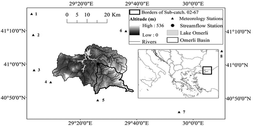
Table 1. Meteorological stations around the Omerli basin and their relevant geographical information.
Figure 2. Flowchart of the methodology used.
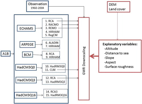
Table 2. Explanatory variables used in the GWR application (C: combination, VAR: variable).
Figure 3. (a) Mean RMSE and (b) bias ratio values calculated from GWR-simulated monthly precipitation at meteorological stations for 16 GWR combinations.
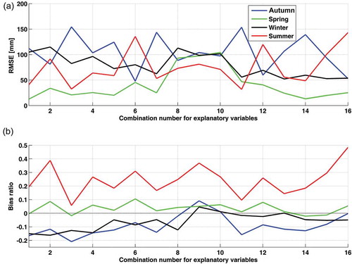
Table 3. Calculated median values of explanatory variables for 16 RCM grids in the GWR application.
Figure 4. The 16 numbered 25-km RCM grids around the Omerli basin and 1-km GWR prediction grids within the sub-catchment. The locations of meteorological stations are also shown.
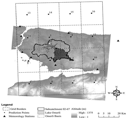
Figure 5. Comparisons between observed and simulated daily precipitation averaged over the reference period for each of the GCM/RCM combinations. Precipitation time series are shown with their 1-day and 30-day moving averages. Each figure panel belongs to an individual model. Subplots identified with some models (1, 2, 3, 11 and 12) also show the corresponding precipitation time series according to GWR application.
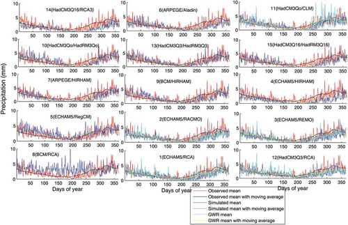
Figure 6. Daily simulated precipitation, with and without GWR, averaged over five RCMs for a 30-day moving window compared with observed precipitation.
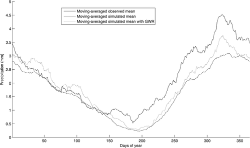
Table 4. Mean RMSE, bias, bias ratio and standard deviation (SD) of each model pair calculated from a 30-day moving-average data series and the reference period. Underlined bold characters represent values from the HIRHAM RCM initialized by ECHAM5, ARPEGE and BCM (4, 7, 9); italic bold characters represent statistics for the RCA model initialized by ECHAM5, BCM and HadCM3Q3 (1, 8, 12). Other models (1–5, 6–7, 8–9, 10–11, 12–13, 14–15) provide values from different regional climate models initiated by the same GCM. The values in parentheses are from the GWR method applied to the specific RCM model.
Figure 7. Monthly mean precipitation of five RCMs compared with observed precipitation averaged (a) over the reference period for original RCMs, and (b) for downscaled RCM precipitation. Standard deviations for five models for monthly mean precipitation are also indicated.
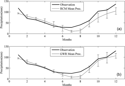
Figure 8. Box plots of extreme precipitation indexes from five RCMs for five different search windows for winter (DJF), spring (MAM), summer (JJA) and autumn (SON), as well as all year, for (a) a 1-year return level, and (b) a 5-year return level; and equivalent plots using a GWR method for (c) a 1-year level, and (d) for a 5-year level. Search windows from left to right are for 1, 2, 5, 10 and 30 days. On each box, the central mark represents the median; the lower and upper edges of the box are the 25th and 75th percentiles, respectively. The whiskers extend to the most extreme data points that are not considered outliers; outliers are shown as plus signs. The whisker length is 1.5 (default value).
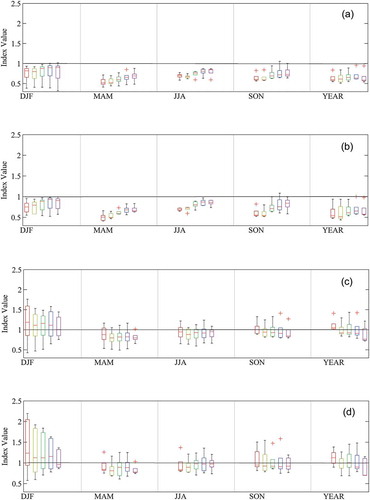
Figure 9. Index values of extreme precipitations from five RCMs for five different search windows for winter (DJF), spring (MAM), summer (JJA) and autumn (SON), as well as all year, for (a) a 1-year level, and (b) a 5-year level; and equivalent plots using a GWR method for (c) a 1-year level, and (d) a 5-year level. Search windows from left to right are for 1, 2, 3, 10 and 30 days.
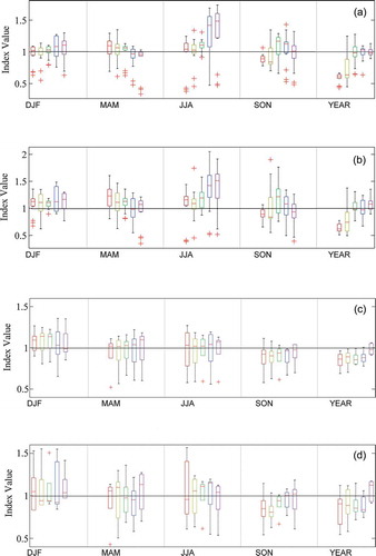
Figure 10. Probability of non-exceedence vs daily precipitation for observations and 15 RCMs for (a) the reference period, and (b) the future period. The observed frequency curve (bold, blue dots) is given in the future period as a baseline.
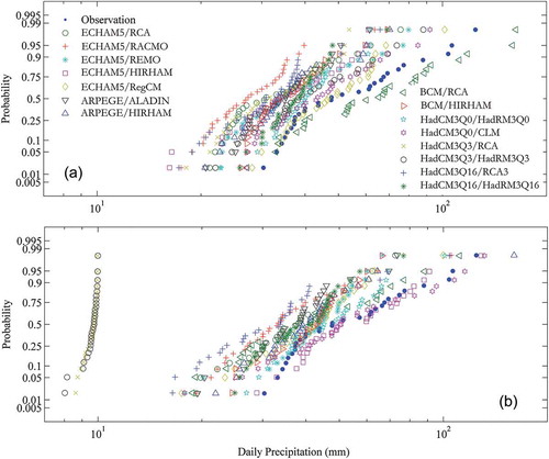
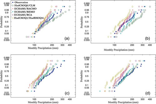
Figure 11. Probability of non-exceedence vs maximum monthly precipitation for observations and five downscaled RCMs for (a) the reference period and (b) the future period, with equivalent plots from the original five RCMs for (c) the reference period and (d) the future period. The observed frequency curve (bold, blue dots) is given in the future period as a baseline.