Figures & data
Figure 1. Sample scheme for a possible model set-up. The model is embedded in a Monte Carlo framework to detect worst-case spatio-temporal precipitation distributions.
Figure 2. Examples of randomly generated (a) spatial precipitation distribution, with each shade representing a meteorological region, and (b) cumulative temporal precipitation distribution, for the entire catchment.
Figure 3. Observed annual maximum floods of the Aare River at Bern.
Figure 4. (a) The Aare basin at the northern edge of the Swiss Alps. (b) Division of the study area into three meteorological regions: A (East, 1145 km2), B (West, 1265 km2) and C (North, 525 km2), with each meteorological region further divided into four or five catchments. (Data: Federal Office of Topography swisstopo)
Figure 5. AQD curves generated by Grebner and Roesch (Citation1998) for different event durations: (a) the dashed curve (72 h) was generated using the area-dependent quotient between the 48 h-curve and the 72 h-curve of the measured data. (b) Curves with the highest observed values in the study area.
Figure 6. Observed spatial and temporal precipitation distributions of the 2005 flood event compared with the best reconstruction out of 10 000 valid generated distributions.
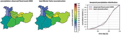
Figure 7. Measured and simulated hydrographs for the 2005, 2007 and 1987 events. The dashed line represents the model run with the observed precipitation data; the thin grey lines represent model runs with redistributed event precipitation and indicate the sensitivity of the model to the spatio-temporal precipitation distribution. The unit hydrographs were generated based on the 2005 event; hence it can be viewed as a calibration event.
Figure 8. Example of the generated hydrographs for the event duration of 72 h. The single hydrographs represent the various spatio-temporal precipitation distributions as discussed in Section 4.
Figure 9. Range of peak discharges of each modelled hydrograph compared with the FOEN (Citation2009) results and the envelope curve by Weingartner (Citation1999). The points indicate the highest ever observed events for the Aare–Bern basin as well as for smaller catchments within the basin. The boxplot to the far right represents the variation of catchment reactions to a given worst-case input due to varying spatio-temporal precipitation distributions.
Figure 10. Range of the modelled peak discharges of model runs in which a particular catchment obtained an extremely high or low precipitation fraction. The peak discharge refers to the whole basin, e.g. the boxplot on the far left shows the distribution of the peak discharges of the whole basin resulting from all model runs in which the catchment A1 received a relatively high precipitation fraction.
Figure 11. Median peak discharges from model runs in which the temporal precipitation distribution was congruent with the respective sector.