Figures & data
Figure 1. Locations and names of meteorological stations used in this study.
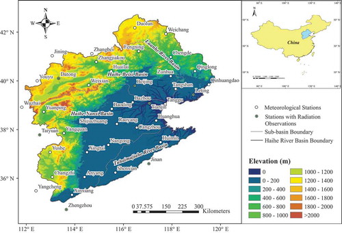
Table 1. Comparison of four different measures between monthly observed ET0 and NCEP-downscaled results for HadCM3 and CGCM3 of the basin average during calibration (January 1961–December 1990) and validation (January 1991–December 2000). The values in brackets represent the measures without post bias correction.
Figure 2. Comparison of monthly ET0 for yearly basin averages from the observed results and the NCEP-downscaled results for HadCM3 and CGCM3: (a) calibration period (January 1961–December 1990) and (b) validation period (January 1991–December 2000).
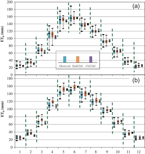
Figure 3. Comparison of long time ET0 series for the basin average from the observed results and the NCEP-downscaled results for both GCMs (solid lines and dashed lines represent the results with or without post bias correction, respectively) in the calibration and validation periods: (a) annual, (b) spring, (c) summer, (d) autumn and (e) winter.
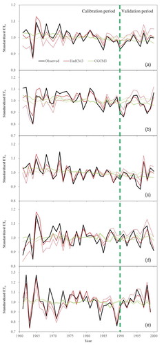
Table 2. Variance contributions (%) to annual ET0 before and after rotating the first four principal components under the H3A2 scenario.
Figure 4. First four REOF modes of annual ET0 during 2011–2099 under the H3A2 scenario with about 92.4% of total variation: (a) first mode with about 48.9% of total variation, (b) second mode with about 23.4% of total variation, (c) third mode with about 10.6% of total variation, and (d) fourth mode with about 9.5% of total variation.
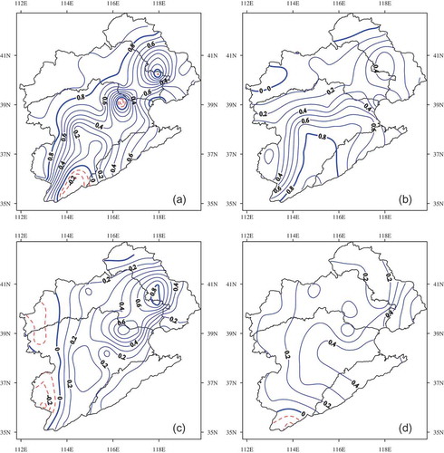
Figure 5. Meteorological stations and homogenous regions obtained by the REOF analysis on the Haihe River Basin.
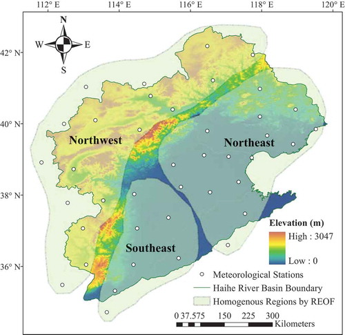
Figure 6. Change points and segmented trends of ET0 for the different homogeneous regions during 2011–2099 under the H3A2 and H3B2 scenarios. Dots denote the ET0 values; solid black lines denote the trend by segmented regression; dashed (red) lines denote the trend by the simple linear regression and the vertical (green) lines give the locations of change points.
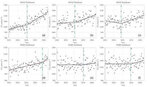
Table 3. Change points (bold) of averaged ET0 for each sub-region during 2011–2099 under the H3A2 and H3B2 scenarios; the trend slopes (unit: mm year−1) of ET0 before and after the change points are listed in parentheses. The dominant climatic variables by multiple stepwise regression are also shown.
Figure 7. Variations of ET0 series for the basin average at annual and seasonal scales under (a) the H3A2 scenario and (b) the H3B2 scenario.
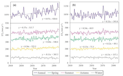
Figure 8. Change rates (%) in annual and seasonal ET0 for three different homogeneous regions: (a) Northwest, (b) Northeast and (c) Southeast, between the baseline period (1961–1990) and the future period (2011–2099) under the H3A2 and H3B2 scenarios.