Figures & data
Figure 1. Location of the USGS stream gauges used in this study.
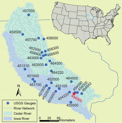
Figure 2. Schematic of selecting recession segments from a complete recession curve by fixing the length while varying the starting points (upper panels) and by fixing the starting point while varying the lengths (lower panels). The insets are the associated dQ/dt vs Q plots following the VTS method and the straight lines in these plots are the regression lines. The starting point of a recession segment is measured from the hydrograph peak marked by the red dashed line. The blue curve is the recession segment used to estimate the recession parameters A and B. This is a 27-day complete recession curve observed at Clear Creek near Coralville, Iowa (USGS 454300), for 24 June 2007 until 19 July 2007.
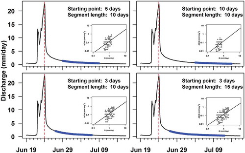
Figure 3. Variability of B estimates due to the change in starting point of recession segments (a single event). The same example recession event as in is used here. Key shows length of recession segments used to estimate B.
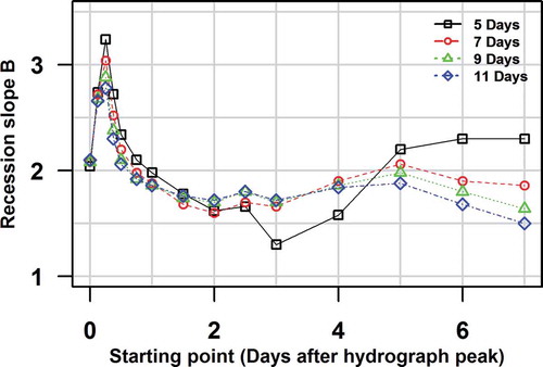
Figure 4. Variability of B estimates due to the change in starting points of recession segments (multiple events). For each USGS gauge (see gauge ID at the top right corner), we repeated the analysis in to obtain ΔB values for all of the recession events. Each red dot is the median value and each grey line segment represents the range of ΔB at a fixed recession length. The median values of ΔB for all gauges are around 1.0.
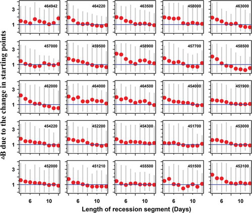
Figure 5. Variability of B estimates due to the change in length of recession segments (a single event). The same example recession event as in is used here. The text at the top right corner is the starting point (number of days after hydrograph peak) of the recession segments used to estimate B.
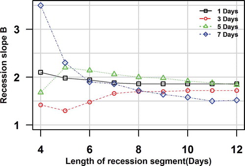
Figure 6. Variability of B estimates due to the change in length of recession segments (multiple events). For each USGS gauge (see gauge ID at the top right corner), we repeated the analysis in to obtain ΔB values for all of the recession events. Each red dot is the median value and each grey line segment represents the range of ΔB at a fixed starting point. The median values of ΔB for all gauges are around 0.5.
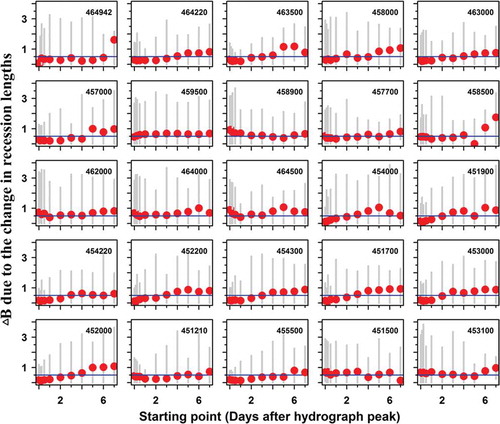
Figure 7. Variability of parameter estimates due to method choices. The same example recession event as in is used here. The parameters for the selected segment were estimated using the CTS (a) and (c), VTS (b) and (d) and NDF (e) methods. In (b), (d) and (e), open circles are measured streamflow values, and lines are the modelled recession segments using the estimated parameters.
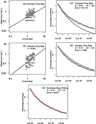
Table 1. Comparison of estimates of recession parameters A and B at Clear Creek near Coralville, Iowa (USGS 454300), calculated using the CTS, VTS and NDF methods. All recession segments have a starting point of 2 days and a length of 7 days.
Table 2. Comparison of the estimates of B at 25 gauges calculated with the CTS, VTS and NDF methods. All gauges are located within the HUC05 of the United States, and we use only the last six digits of their complete USGS gauge ID. NRec is the number of recession events analysed; Medians of B are the median values of B for multiple events at a gauge; IQR of B is the interquartile range of B estimates for multiple events at a gauge; modelling error (%) is the median of the relative differences between the volumes of modelled and observed recession flows; p value is for the paired t-test; and ∆B is the median value of absolute difference of B estimates given by two methods.
Figure 8. Robustness of the VTS (blue) and the NDF (red) methods with respect to the noise in streamflow data. The true value of B is 2. Filled circles represent the mean values of B. Error bars show the standard deviation of B estimates at each magnitude of error.
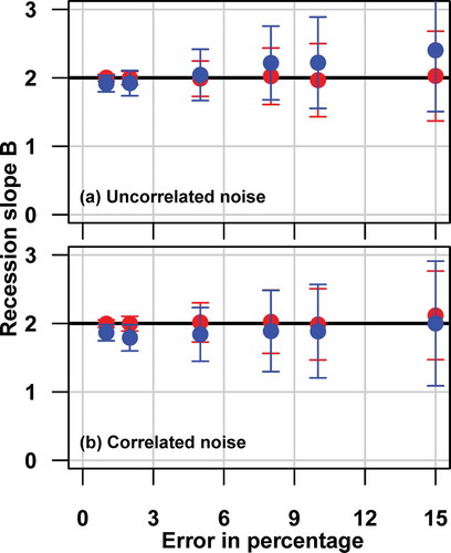
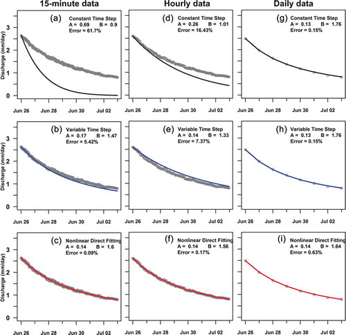
Figure 9. Comparison of A and B estimated using three methods and streamflow data with three temporal resolutions (dt = 15 min, 1 h, and 1 day were used to calculate dQ/dt). The same example recession event as in is used here. We extracted the recession segment from the complete recession curve using a starting point of 2 days and a length of 7 days. The open circles are the observed streamflow values, and the lines are the modelled recession segments using the estimated parameters. For the VTS method, the value C = 0.001 was used to reduce the impact of the noise in streamflow data on the estimation of recession parameters.