Figures & data
Figure 1. Schematic representation of a sequence of runs with examples of total deficit, duration, mutually dependent events and minor events. Discharge (Q) is shown as a grey line and the low-flow threshold (Q95) as a black line.
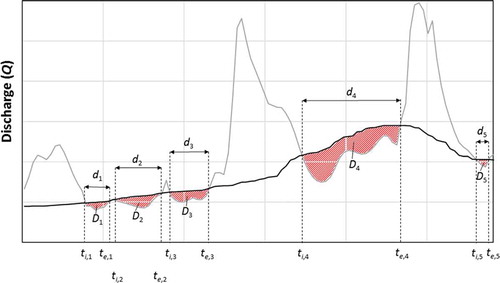
Figure 2. Flowchart describing the computational scheme for the implementation of the proposed low-flow index into an operational monitoring system. The variables Q95,t and λ are derived from the historical baseline dataset as described in the text, and the initial conditions are defined as D0 = d0 = 0 and g0 = ∞.
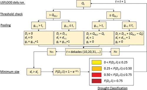
Figure 3. Example of time series of daily discharge (grey line) and low-flow threshold (black lines) for two rivers: Imera Meridionale (13.9265E, 37.1618N; upper panel) and Upper Danube (18.8866E, 47.2040N; lower panel).
Table 1. Summary of the European average characteristics of the total deficit partial duration series for the period 1995–2013.
Figure 4. Spatial distribution of the number of events (left panel) and average length of the runs (right panel) in the period 1995–2013.
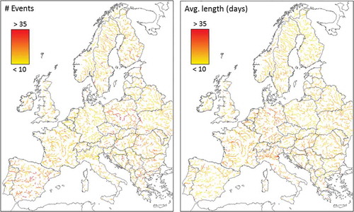
Figure 5. Four examples of near real-time monitoring of hydrological drought with the SRI (upper line) and the proposed index (lower line). Each SRI time series represents the monthly values classified as follows: −0.84 to −1.00: yellow, −1.01 to −1.50: orange, −1.51 to −2.00: red, <−2.00: maroon (see Agnew Citation2000); the FD time series are the dekadal values classified with the following colour scheme: mild: yellow, moderate: orange, severe: red, extreme: maroon (see ).
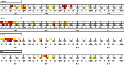
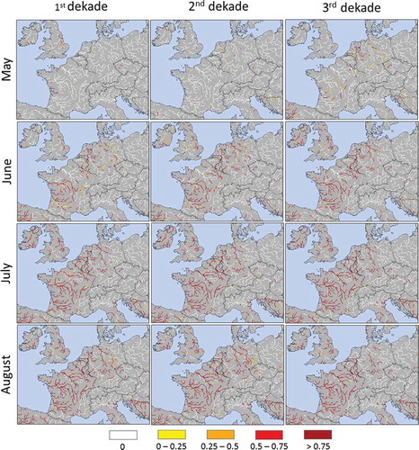
Figure 6. Sequence of FD dekadal maps for summer (May–August) 2015 in Central Europe. The land cells with drainage area <1000 km2 are depicted in grey; the main rivers are coloured according to the scheme: no-drought: white, mild: yellow, moderate: orange, severe: red, extreme: maroon (see ).