Spatio-temporal downscaling of projected precipitation in the 21st century: indication of a wetter monsoon over the Upper Mahanadi Basin, India

Figures & data

Figure 1. Schematic diagram of data used and the methodology adopted.

Figure 2. Map showing the Mahanadi Basin (key map) and the Upper Mahanadi Basin (UMB, highlighted and enlarged). Gridded locations for downscaling grid intersections (circles) and GCM grid intersections (triangles) are also shown in the enlarged UMB. Nine grid intersections are also considered for CanESM2, in which the study area is enclosed. These are not shown for clarity. A digital elevation model (DEM) of the study basin is shown in greyscale (m a.m.s.l.).

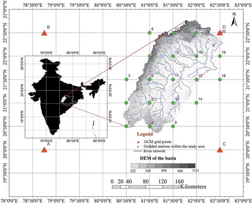
Table 1. Predictor variables from NCEP re-analysis and HadCM3 datasets, and frequency of being selected based on high correlation coefficient with observed precipitation in the Upper Mahanadi Basin.

Predictor code	Description	Frequency of use
mslp	Mean sea level pressure	18/20
P5_u	500 hPa zonal velocity	18/20
P500	500 hPa geopotential height	18/20
shum	1000 hPa specific humidity	17/20
P8_v	850 hPa meridional velocity	17/20
r850	850 hPa relative humidity	17/20
P850	850 hPa geopotential height	16/20
P_u	1000 hPa zonal velocity	12/20
P5th	500 hPa wind direction	10/20
P5_v	500 hPa meridional velocity	8/20
r500	500 hPa relative humidity	3/20
P_v	1000 hPa meridional velocity	2/20
P8th	850 hPa wind direction	1/20

Figure 3. Calibration and validation results of statistical downscaling model (SDSM) with NCEP re-analysis predictors for location 12, marked in Figure 2. Observed and downscaled precipitation during calibration at (a) the daily scale and (b) the monthly scale. (c) Scatter plot at the monthly scale during calibration (RMSE: 1.935 mm, R²: 0.757, and NSE: 0.745). Observed and downscaled precipitation during validation at (d) the daily scale and (e) the monthly scale. (f) Scatter plot at the monthly scale during validation (RMSE: 1.976 mm, R²: 0.780, NSE: 0.753).

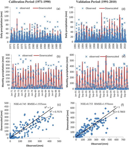
Figure 4. Calibration and validation results of SDSM at location 12, marked in Figure 2 using CanESM2 outputs. Observed and downscaled precipitation during calibration at (a) the daily scale and (b) the monthly scale. (c) Scatter plot at the monthly scale during calibration (RMSE: 2.450 mm, R²: 0.733, and NSE: 0.652). Observed and downscaled precipitation during validation at (d) the daily scale and (e) the monthly scale. (f) Scatter plot at the monthly scale during validation (RMSE: 2.240 mm, R²: 0.764, NSE: 0.719).

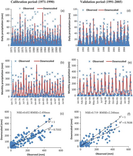
Table 2. Statistical performance measures between observed and downscaled (by SDSM) precipitation for the calibration and validation periods at all locations using HadCM3 outputs as input to SDSM.

		Calibration			Validation
Location no.	Location	RMSE (mm)	R^2	NSE	RMSE (mm)	R^2	NSE
1	20.5°N, 80.5°E	2.82	0.61	0.58	3.11	0.64	0.63
2	21.0°N, 80.5°E	2.92	0.64	0.61	2.99	0.66	0.65
3	21.0°N, 80.5°E	3.24	0.60	0.57	3.16	0.60	0.58
4	20.5°N, 81.0°E	3.06	0.71	0.71	3.08	0.70	0.69
5	21.0°N, 81.0°E	2.81	0.67	0.67	2.94	0.64	0.60
6	21.5°N, 81.0°E	2.05	0.71	0.69	2.05	0.67	0.58
7	22.0°N, 81.0°E	2.41	0.71	0.68	2.43	0.68	0.67
8	22.5°N, 81.0°E	3.13	0.65	0.57	2.98	0.66	0.61
9	20.5°N, 81.5°E	2.72	0.64	0.64	2.86	0.67	0.64
10	21.0°N, 81.5°E	2.42	0.67	0.70	2.41	0.70	0.70
11	21.5°N, 81.5°E	2.37	0.68	0.66	2.37	0.76	0.74
12	22.0°N, 81.5°E	1.94	0.76	0.75	1.98	0.78	0.75
13	22.5°N, 81.5°E	2.27	0.75	0.74	1.64	0.81	0.79
14	21.0°N, 82.0°E	3.17	0.72	0.69	2.96	0.69	0.67
15	21.5°N, 82.0°E	2.40	0.72	0.70	2.36	0.69	0.66
16	22.0°N, 82.0°E	2.47	0.70	0.70	2.16	0.75	0.74
17	22.5°N, 82.0°E	2.31	0.75	0.74	2.11	0.74	0.71
18	21.5°N, 82.5°E	3.05	0.68	0.64	3.22	0.67	0.65
19	22.0°N, 82.5°E	2.40	0.77	0.77	2.73	0.66	0.64
20	22.5°N, 82.5°E	2.34	0.73	0.71	2.15	0.78	0.74

Table 3. Statistical performance measures between observed and downscaled (by SDSM) precipitation for the calibration and validation periods at different locations using CanESM2 outputs as input to SDSM.

		Calibration			Validation
Location no.	Location	RMSE (mm)	R^2	NSE	RMSE (mm)	R^2	NSE
1	20.5°N, 80.5°E	3.29	0.65	0.62	3.21	0.66	0.64
2	21.0°N, 80.5°E	3.12	0.61	0.60	2.90	0.64	0.63
3	21.0°N, 80.5°E	2.86	0.68	0.66	3.17	0.61	0.61
4	20.5°N, 81.0°E	3.18	0.70	0.65	3.24	0.67	0.64
5	21.0°N, 81.0°E	3.12	0.62	0.61	2.83	0.69	0.67
6	21.5°N, 81.0°E	2.43	0.65	0.61	2.62	0.62	0.58
7	22.0°N, 81.0°E	2.03	0.70	0.70	2.31	0.68	0.62
8	22.5°N, 81.0°E	2.83	0.71	0.64	3.16	0.68	0.65
9	20.5°N, 81.5°E	3.05	0.60	0.60	2.87	0.70	0.62
10	21.0°N, 81.5°E	2.66	0.62	0.61	2.48	0.67	0.62
11	21.5°N, 81.5°E	2.43	0.65	0.62	2.17	0.68	0.66
12	22.0°N, 81.5°E	2.45	0.73	0.65	2.24	0.76	0.72
13	22.5°N, 81.5°E	2.73	0.70	0.65	2.56	0.69	0.68
14	21.0°N, 82.0°E	2.97	0.68	0.60	2.87	0.70	0.62
15	21.5°N, 82.0°E	2.63	0.67	0.59	2.47	0.70	0.62
16	22.0°N, 82.0°E	3.11	0.68	0.61	3.00	0.70	0.63
17	22.5°N, 82.0°E	2.86	0.71	0.62	2.37	0.74	0.69
18	21.5°N, 82.5°E	2.97	0.62	0.61	2.68	0.67	0.61
19	22.0°N, 82.5°E	2.98	0.66	0.59	2.67	0.73	0.66
20	22.5°N, 82.5°E	3.02	0.70	0.65	2.89	0.74	0.69

Table 4. Month-wise bias correction factors for HadCM3 A2 and B2 scenarios and CanESM2.

	HadCM3 Scenarios
Month	A2	B2	CanESM2
January	0.58	0.53	1.35
February	0.66	0.56	1.52
March	1.02	0.64	0.74
April	0.48	0.63	0.56
May	0.49	0.52	0.61
June	0.79	0.87	0.83
July	1.14	1.07	1.07
August	0.86	0.87	0.84
September	0.95	0.86	1.12
October	0.49	0.49	0.83
November	0.45	0.49	0.57
December	0.78	0.74	0.54

Figure 5. Annual cycles of Upper Mahanadi Basin precipitation averaged over the entire basin for the period 1971–2010 using downscaled A2 (DS A2) and downscaled B2 (DS B2) scenarios and for 1971–2005 using downscaled CanESM2 (DS CanESM2): (a) observed and downscaled monthly averaged precipitation and (b) standard deviation.

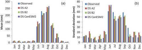
Figure 6. Box plots of (a) observed, (b) downscaled HadCM3 A2 scenario and (c) downscaled HadCM3 B2 scenario precipitation distributions for all locations in the study basin during the period 1971–2010. (d) Downscaled CanESM2 precipitation distribution for the study basin during the period 1971–2005.

Figure 7. Comparison of downscaled precipitation with baseline (1971–2000) precipitation: (a) HadCM3 (A2 scenario) precipitation, (b) HadCM3 (B2 scenario) precipitation and (c) CanESM2 (RCP 4.5) precipitation.

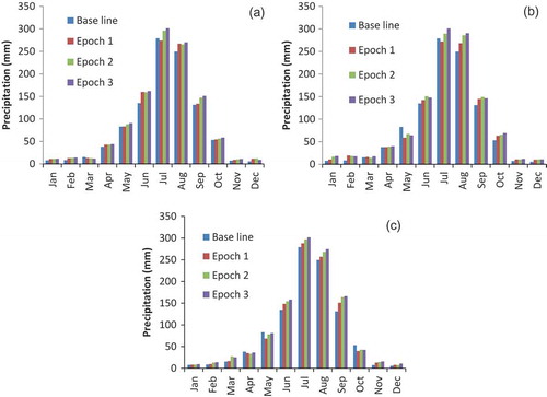
Figure 8. Daily extremes for all months between observed precipitation during the baseline period (1971–2000), bias corrected, downscaled precipitation for HadCM3 A2 and B2 emissions scenarios for epoch-3 (2071–2099) and CanESM2 (RCP4.5) for epoch-3 (2071–2100), respectively shown as 1, 2, 3 and 4 on the x-axis. The boxes represent the 25th, 50th and 75th quantiles.

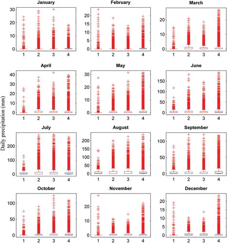
Table 5. Precipitation magnitude (in mm) corresponding to the 95th quantile for baseline and future epochs.

	Projected future precipitation
	HadCM3
	A2 scenario			B2 scenario			CanESM2
Baseline	Epoch-1	Epoch-2	Epoch-3	Epoch-1	Epoch-2	Epoch-3	Epoch-1	Epoch-2	Epoch-3
17.26	22.88	24.14	24.31	23.05	24.25	24.48	21.35	22.01	23.51

Table 6. Month-wise variation of 95th quantile of daily precipitation (in mm).

		A2 scenario			B2 scenario			Can ESM2
Month	Observed	Epoch-1	Epoch-2	Epoch-3	Epoch-1	Epoch-2	Epoch-3	Epoch-1	Epoch-2	Epoch-3
January	2.26	2.75	2.83	2.71	2.39	2.72	2.13	2.17	2.15	2.22
February	2.37	2.26	2.31	2.21	1.92	2.00	1.95	2.36	2.39	2.33
March	1.58	4.70	4.79	4.67	3.64	3.62	3.70	5.01	4.70	5.44
April	1.27	7.66	8.07	7.42	6.81	6.58	6.79	6.74	6.98	7.09
May	2.29	4.39	4.70	4.40	5.28	5.51	5.21	6.24	6.79	7.10
June	22.26	40.07	40.07	39.60	46.82	46.81	44.12	28.50	30.76	36.54
July	34.69	76.95	79.68	80.32	81.49	82.95	83.9	43.84	48.80	58.41
August	38.05	56.86	56.45	55.04	54.12	56.01	53.41	38.77	44.22	50.35
September	21.56	36.46	37.84	38.89	35.31	35.63	34.27	27.53	30.90	32.91
October	9.21	17.31	17.36	15.71	19.12	19.16	19.97	16.35	17.69	21.21
November	2.07	2.64	2.59	2.49	2.58	2.56	2.59	3.20	3.00	3.73
December	0.71	2.91	2.84	2.84	3.44	3.37	3.63	2.351	2.50	2.76

Table 7. Number of events with rainfall greater than the baseline 95th quantile value (in %).

		A2 scenario			B2 scenario			CanESM2
Month	Observed	Epoch-1	Epoch-2	Epoch-3	Epoch-1	Epoch-2	Epoch-3	Epoch-1	Epoch-2	Epoch-3
January	5.05	5.80	6.00	6.16	5.28	5.84	5.01	4.79	4.71	4.89
February	5.00	4.73	5.12	4.80	3.98	4.18	4.10	4.99	5.23	4.92
March	5.05	21.17	20.89	20.23	16.41	15.82	16.28	14.50	13.37	14.70
April	5.00	27.47	29.02	26.55	24.44	24.24	24.16	19.64	19.42	20.70
May	5.05	11.74	12.57	11.71	13.60	14.48	13.32	13.12	14.05	15.05
June	5.00	14.10	15.13	14.37	14.50	15.11	13.21	6.69	7.20	8.85
July	5.05	16.31	16.87	17.22	16.36	16.52	14.57	6.74	7.29	9.03
August	5.05	9.99	10.09	9.26	9.09	9.44	9.15	5.15	6.11	6.77
September	5.00	10.89	11.28	11.70	10.09	10.93	10.44	6.70	7.53	9.13
October	5.05	11.17	10.86	10.28	11.77	12.45	13.01	8.77	9.68	12.07
November	5.00	7.71	7.24	7.17	7.13	7.28	7.49	7.74	7.39	8.68
December	4.85	28.47	28.79	28.43	27.41	26.09	27.74	13.24	13.98	15.42