Correcting bias in rainfall inputs to a semi-distributed hydrological model using downstream flow simulation errors

Figures & data

Figure 1. Sub-basins and streamflow gauging stations of the Okavango River basin (ignoring three small stations to the east of Serpa Pinto).

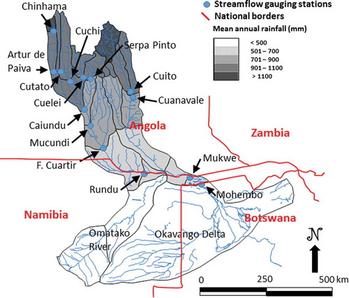
Figure 2. (a) Flow duration curves and (b) time series of simulated and observed annual stream volumes at the outlet of the Rundu sub-basin.

Table 1. Form and parameters of the relationships between runoff coefficient and rainfall index.

Sub-basin/downstream reference	Equation form	A	B	R^2
Chinhama/Rundu	Exponential	0.0951	0.6881	0.888
Artur de Paiva/Rundu	Exponential	0.032	1.1409	0.875
Cutato/Rundu	Exponential	0.0393	1.0253	0.857
Cuchi/Rundu	Exponential	0.0209	1.2319	0.841
Cuelei/Rundu	Exponential	0.0246	1.073	0.722
Caiundo/Rundu	Exponential	0.002	2.2255	0.761
Serpa Pinto/Rundu	Linear	0.0648	0.0296	0.233
Mucundi/Rundu	Linear	−0.1081	0.1001	0.674
F. Cuartir/Rundu	Linear	−0.0262	0.031	0.550
Northeast/Mukwe	Linear	0.2244	−0.0174	0.072
Cuito/Mukwe	Linear	0.2295	−0.0581	0.411
Cuanavale/Mukwe	Linear	0.0913	−0.0028	0.004

Figure 3. Examples of the relationship between the rainfall index and simulated runoff ratio for (a) Chinama, (b) Caiundo, (c) Serpa Pinto and (d) Cuanavale sub-basins.

Figure 4. Illustration of the part of the approach used to adjust the input rainfall data using relationships between an index of annual rainfall (total depth + maximum monthly depth) and simulated runoff ratio.

Figure 5. Comparison of relationships between the rainfall index and simulated runoff ratio for five sub-basins using the total time series (94 years: black lines) and using only the first 47 years (grey lines).

Table 2. Model performance indices (ranges of objective functions across all 10 000 ensembles) before and after rainfall corrections. CE: Nash-Sutcliffe coefficient of efficiency (untransformed data); CE{ln}: Nash-Sutcliffe coefficient of efficiency (ln transformed data); %Bias: % bias in the simulated mean monthly flow relative to the observed mean.

			Objective function statistic ranges for all ensembles (CE, CE{ln}, %Bias)
Sub-basin	Cumulative area (km^2)	No. of upstream sub-basins	Original rainfall	Corrected rainfall
Chinhama	1 822	0	0.321 to 0.596	0.503 to 0.715
			0.601 to 0.765	0.486 to 0.839
			–6.8 to 14.0	–20.3 to −0.6
Artur de Paiva	7 153	1	0.228 to 0.587	0.471 to 0.737
			0.564 to 0.713	0.616 to 0.817
			–4.6 to 27.6	–16.2 to 14.0
Cutato	3 621	0	0.177 to 0.524	0.359 to 0.674
			0.416 to 0.602	0.308 to 0.648
			–14.9 to 2.5	–23.0 to −6.7
Cuchi	10 594	0	0.288 to 0.599	0.489 to 0.739
			0.585 to 0.732	–0.215 to 0.774
			–1.6 to 9.1	–11.6 to −0.5
Cuelei	5 466	0	0.628 to 0.734	0.569 to 0.674
			0.640 to 0.823	0.538 to 0.847
			–11.8 to 9.9	–24.5 to −4.3
Caiundo	38 440	4	−0.005 to 0.553	0.329 to 0.621
			0.457 to 0.650	0.445 to 0.673
			–6.5 to 42.2	–18.5 to 23.5
Mucundi	50 721	7	0.123 to 0.723	0.448 to 0.816
			0.723 to 0.787	0.648 to 0.845
			–2.3 to 45.1	–10.6 to 30.6
F. Cuartir	71 280	8	0.437 to 0.833	0.628 to 0.887
			0.698 to 0.883	0.777 to 0.926
			–4.7 to 36.4	–12.2 to 28.1
Rundu	95 662	9	0.228 to 0.644	0.448 to 0.849
			0.551 to 0.803	0.605 to 0.893
			–6.7 to 34.3	–7.3 to 34.3
Cuito	15 857	1	0.169 to 0.564	0.174 to 0.573
			–0.119 to 0.548	–0.133 to 0.561
			–14.4 to −5.5	–14.8 to −5.4
Cuanavale	23 347	2	0.278 to 0.793	0.232 to 0.774
			0.406 to 0.796	0.402 to 0.789
			–2.5 to 10.0	–2.6 to 10.0
Mukwe	226 256	22	0.206 to 0.609	0.420 to 0.752
			0.560 to 0.715	0.623 to 0.783
			–1.3 to 23.8	–1.8 to 23.9
Mohembo	228 798	23	0.039 to 0.619	0.167 to 0.754
			0.515 to 0.754	0.515 to 0.814
			3.5 to 30.2	5.6 to 33.3

Figure 6. Monthly time series comparisons between observed, and simulated streamflow volumes before and after the rainfall adjustments for four sub-basins: (a) Cuchi, (b) Mucundu, (c) Cuanavale and (d) Rundu.

Figure 7. Example frequency distributions of a combined performance index (CE + CE{ln}, +(1 − abs(%Bias)/100) + (1 − abs(%Bias{ln}/100), having a maximum value of 4.0.

Figure 8. Examples of changes made to the UDEL rainfall data: (a) time series of annual rainfall corrections (see text for explanation); and (b) exceedence frequency curves for monthly rainfall, before and after adjustment.

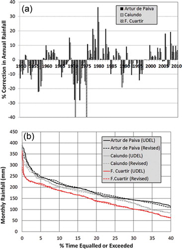
Figure 9. Monthly time series comparisons between observed, and simulated streamflow volumes before and after the rainfall adjustments for Rundu during the most recent data period.