Figures & data
Figure 1. Framework for input uncertainty quantification in Stage 1 of optimization.
Figure 2. Plots of autocorrelation: (a) discharge; and cross-correlation of (b) discharge–rainfall and (c) discharge–evapotranspiration.
Figure 3. The final architecture of ANN identified for the Leaf River basin.
Figure 4. Histogram of rainfall multiplier sampled from the log-normal distribution (Leaf River).
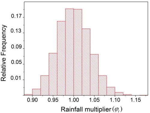
Figure 5. Two-dimensional scatter plots of observed rainfall vs corrected rainfall.
Figure 6. Convergence of objective function against number of generations.
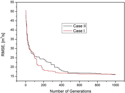
Table 1. Statistical properties of the ANN parameters optimized for Case I and Case II. SD: standard deviation.
Table 2. Summary statistics and model performance indices.
Figure 7. Case I: Variation of parameter range along the number of generations. W: weight parameter; B: bias parameter; I, H and O: input, hidden and output nodes, respectively; subscript i corresponds to the ith node in the respective layer, e.g. WI1H2 indicates a weight connection between 1st input and 2nd hidden node.
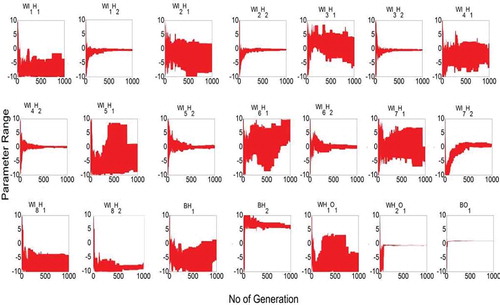
Figure 8. Case II: Variation of parameter range along the number of generations. See for explanation of notation.
Figure 9. Pareto-optimal front of optimization during ensemble creation in the calibration period.
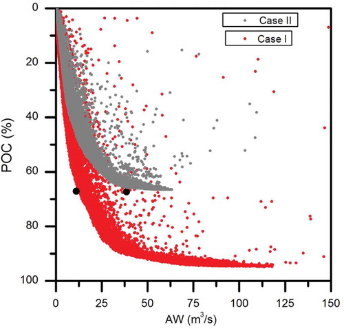
Table 3. Uncertainty indices estimated for Case I and Case II. POC: percentage of coverage; AW: average width.
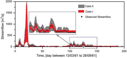
Figure 10. Prediction interval corresponding to selected ensemble during the calibration period.
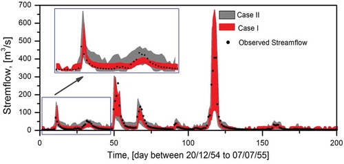
Figure 11. Prediction interval corresponding to selected ensemble during the validation period.