Impact of a low-permeability lens on dune-induced hyporheic exchange

Figures & data

Figure 1. Conceptual illustrations of: (a) theory of Elliott and Brooks (1997a, b); (b)–(d) hyporheic flow (blue dotted line) field and groundwater flow (black dotted line) field beneath the stream bed with dunes under different streamflow conditions (no recharge or discharge, recharge in a losing stream and groundwater discharge in a gaining stream, respectively). Black solid lines in (a) represent the distribution of sinusoidal varied pressures. The black arrows show the flow direction of surface water.

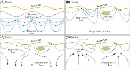
Figure 2. Domain of a numerical model for 2-D dune-induced hyporheic flow. The intervals of vertical and horizontal grid lines were set to 5 mm. The ellipses represent low-permeability lenses. The coordinate system comprises x and z directions, where x represents horizontal location and z the depth of the low-permeability lens. The location of the intermediate source point was set as the origin point (x = 0, z = 0) and the positive directions in x and z were set to be right and downward, respectively. Diamonds represent the distribution of spatial locations of low-permeability lenses.

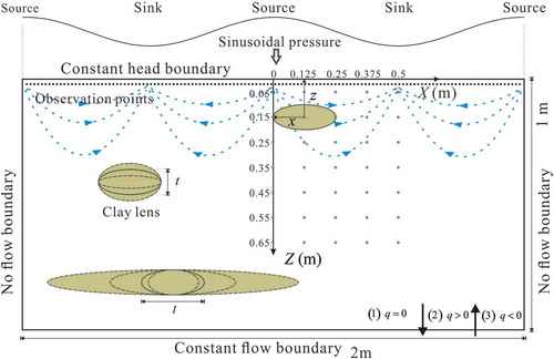
Table 1. Length (l) and thickness (t) of the low-permeability lenses in the numerical experiments.

l (m)	0.2	0.25	0.5	0.25
t (m)	0.1			0.05	0.10	0.15

Figure 3. Schematic of flux flows in and out of the simulated domain at (a) neutral condition, (b) losing condition and (c) gaining condition. The solid arrow refers to hyporheic exchange flux and the dashed arrow represents regional groundwater flux.

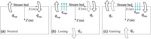
Figure 4. Variation in λ with (a) horizontal location and (b) depth of the low-permeability lens. The dotted line (λ = 1.00) divides two types of effect on hyporheic exchange generated by the low-permeability lens: hindering below the line and enhancement when λ > 1.00.

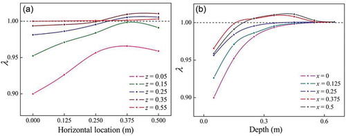
Figure 5. Relationship between spatial location and λ under low-permeability lens of various lengths (l) and thicknesses (t).

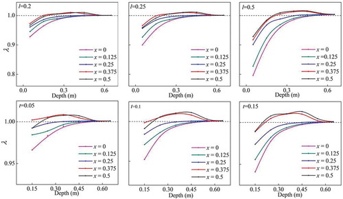
Figure 6. Relationship between intensity of the hyporheic exchange and (a) length of the low-permeability lens and (b) thickness of the low-permeability lens. Horizontal locations of x = 0, 0.125 and 0.25 m were chosen to represent locations from source point to sink point.

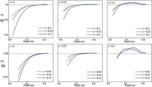
Table 2. Sensitivity coefficient of λ to the length and thickness of the low-permeability lens at various spatial locations.

		x
	z	0.000	0.125	0.250	0.375	0.500
Ul (m^−1)	0.15	−0.215	−0.188	−0.062	−0.067	−0.036
	0.35	−0.030	−0.020	0.011	0.009	0.021
	0.55	0.006	0.007	0.010	0.006	0.018
Ut (m^−1)	0.15	−0.072	−0.085	−0.055	−0.042	−0.009
	0.35	−0.008	−0.008	−0.007	0.004	0.006
	0.55	−0.002	−0.002	−0.001	0.003	0.009

Figure 7. Variation in hyporheic exchange q_hyp versus spatial positions of low-permeability lens under: (a,i) and (b,i) neutral stream; (a,ii) and (a,iii) losing stream; and (b,ii) and (b,iii) gaining stream. The dotted lines in (a) and (b) refer to q_hyp = q₀, i.e. hyporheic exchange in a stream bed without the existence of a low-permeability lens. If q_hyp is above the dotted line, the low-permeability lens enhances the hyporheic process; otherwise, the low-permeability lens hinders hyporheic exchange. The intensity of regional groundwater increases from 0 m d⁻¹ in (a,i) and (b,i) to 0.003 m d⁻¹ in (a,iii) and (b,iii). Part (c) shows the variation trend of λ under q_G = 0, −0.003 and −0.005 m d⁻¹.

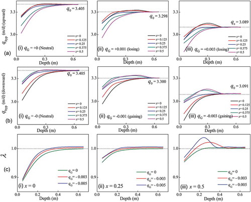
Figure 8. Flow fields of hyporheic exchange controlled by (a) a low-permeability lens with various spatial locations, (b) a lens with various sizes and (c) various intensities of regional groundwater. The ellipse represents a lens; numbers represent the horizontal location and depths of the low-permeability lenses. The hyporheic flow path and regional GW–SW flow path are shown as a dotted line and a dashed line, respectively.

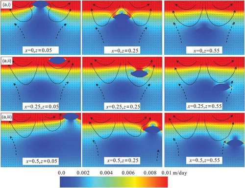
Figure 8. (Continued).

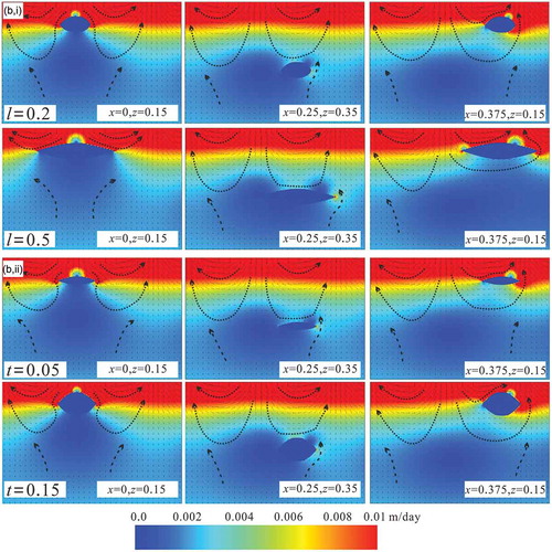
Figure 8. (Continued).

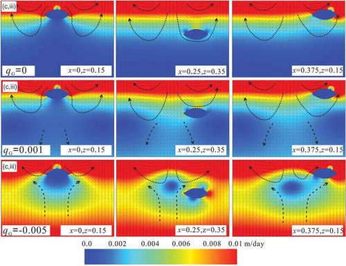
Figure 9. Critical lines controlled by (a) low-permeability lenses of various lengths, (b) low-permeability lenses of various thicknesses, (c) losing condition and (d) gaining condition. The x-coordinate refers to the horizontal location and z the depth of the low-permeability lens.

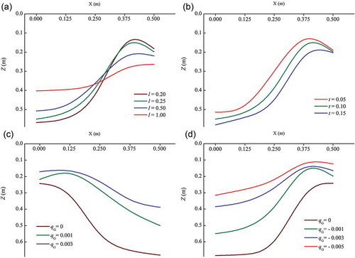
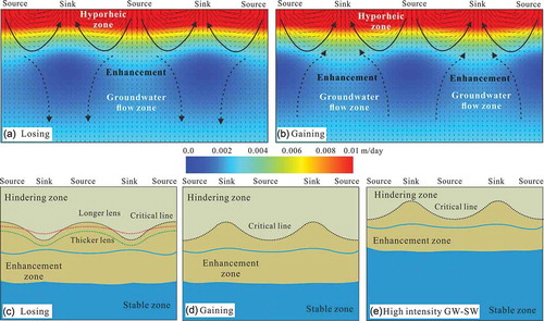
Figure 10. Conceptual illustrations of hyporheic flow fields and regional groundwater flow fields under (a) losing conditions and (b) gaining conditions. Conceptual illustrations of hindering zone, enhancement zone and stable zone under (c) losing condition, (d) gaining condition and (e) regional groundwater of higher intensity. Dotted lines refer to the critical line, where the upper (red) and lower (green) lines represent critical lines under a longer low-permeability lens and a thicker low-permeability lens, respectively. The solid (blue) line refers to the interface of the hyporheic zone.

Elliott, A.H. and Brooks, N.H., 1997a. Transfer of nonsorbing solutes to a streambed with bed forms: laboratory experiments. Water Resources Research, 33, 137–151. doi:10.1029/96WR02783

 Web of Science ®Google Scholar

Elliott, A.H. and Brooks, N.H., 1997b. Transfer of nonsorbing solutes to a streambed with bed forms: theory. Water Resources Research, 33 (1), 123–136. doi:10.1029/96WR02784

 Web of Science ®Google Scholar