
Figures & data
Figure 1. (a) Location of the floodwater spreading (FWS) project in Iran. (b) General view of the study area in Gareh-Bygone Plain (obtained from RGB742 of a Landsat5 image of 21 October 2014). (c) Location of the study site, the second basin of the Bisheh Zard1 (BZ1) FWS (taken from Google Earth, 24 October 2016). W1–W3 are the experimental wells. Black curved lines and black spots are tree plantations. The first upstream earth dike of BZ1 starts from the top right and the flood flows from northeast to southwest.
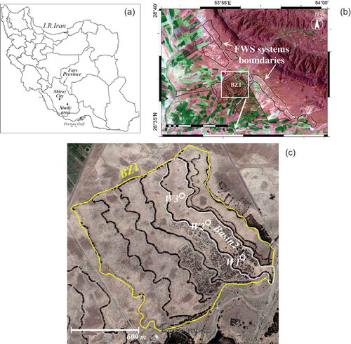
Figure 2. Three-dimensional interpolated map of the sediment depth (cm) of the study area using simple kriging with locally varying mean method. Adapted from Esmaeili-Vardanjani et al. (Citation2013).
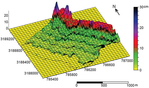
Table 1. Some selected characteristics of the representative layers. Descriptive characteristics of the layers were defined in the field.
Table 2. Vertical distribution of the representative layers (RL) in the wells based on arbitrary coding of the pre-defined characteristics of each RL. The letters A to G were assigned arbitrarily to the representative layers in this study for differentiation and delineation.
Table 3. Statistics of measured field saturated hydraulic conductivity (Kfs, m d−1) of representative layers.
Figure 3. Change in the mean field saturated hydraulic conductivity (Kfs) of the layers due to change in soil texture and stoniness. The lines are regressions between Kfs and corresponding parameters clay+silt (dashed line) and stoniness (solid line).
Figure 4. Soil water content time series for selected depths below ground level (measured by the calibrated TDR probes) and simultaneous rain and flood depth. Layer depths are noted in each graph. Flood data are the depths of pounded water after each flooding event in the system.
Figure 5. Change in the SWC of layers before and after the two flooding events of (a) and (b) 28 January 2011, and (c) and (d) 1 August 2013. Graphs (a) and (c) show the change in SWC for the entire 28-m profile, while graphs (b) and (d) zoom in on the first 5 m of the profile to better illustrate the redistribution of the SWC in the top layers.
Table 4. Soil water balance calculated for the top 4.0 m of layers after the flooding event on 16 January to 23 July 2011 (dates as MM/DD/YY).
Table 5. Statistics of the modified van Genuchten (MVG) model for the representative layers.
Figure 6. Retention curves for the representative layers of Well 1 in the Bisheh Zard FWS system. A: soil surface loam, 7% fine gravel; B: loamy sand, 22% gravel; C: sandy loam, 54% medium gravel; D: sandy loam, 67% coarse gravel; E: sandy loam, 7% fine gravel; F: sand, 53% medium gravel; G: loamy sand, 0.3% medium gravel.
Figure 7. Sensitivity (Si) of simulated flux modelled by HYDRUS 1D to the deviations in hydraulic parameters of the modified van Genuchten (MVG) model: (a) θr, Kfs and l and (b) θs, α and n. Parameters are presented in two graphs because of different magnitudes. The initial value for n was 1.0 and, as n should not be smaller than 1.0, the deviations of 0.5 and 0.75 resulted in the model failure in convergence.
Table 6. Calibration results of the H1D model. The optimal hydraulic model was determined according to the modified van Genuchten (MVG) model. The layer depths of 0.1, 0.6, 1.8 and 4.0 m correspond to the representative layers (RL) A, B, C and G, respectively.
Figure 8. Observed and simulated soil water content at (a) 0.1 m, (b) 0.6 m, (c) 1.8 m and (d) 4.0 m. R2: coefficient of determination; RMSE: root mean square error. The mass balance error of the optimal run of the model was calculated as 0.6%. The optimal hydraulic model was determined according to the MVG model.
Figure 9. Cumulative recharge simulated by H1D for the period 16 January to 23 July 2011. The dashed line shows the amount of total recharge for the entire period.
Table 7. Error in simulated recharge by HYDRUS 1D (H1D) model compared to soil water balance (SWB) method for the period 16 January–23 July 2011. SD: standard deviation; RMSE: root mean square error.