Multi-hydro hydrological modelling of a complex peri-urban catchment with storage basins comparing C-band and X-band radar rainfall data

Figures & data

Figure 1. Bièvre catchment, Massy sub-catchment, C-band radar and X-band radar locations.

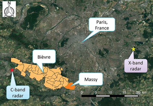
Figure 2. Land use of Massy area with all available layers.

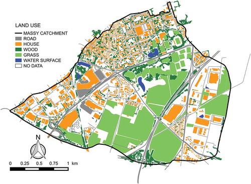
Figure 3. Land use of Massy area: (a) with priority and (b) without priority order.

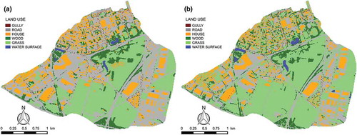
Figure 4. Details of the storm drain system connections.

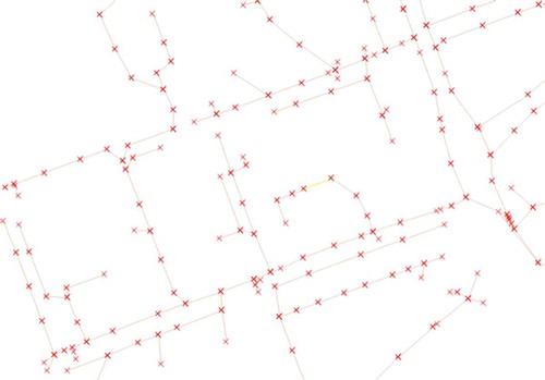
Figure 5. SWMM file of the storm drain system: (a) generated by MH-AssimTool and (b) later corrected.

Figure 6. SWMM file of the Massy sub-catchment and the six storage basins, with the Cora basin (measurement point) highlighted.

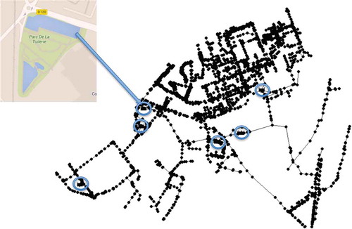
Table 1. Characteristics of the storage basins.

Storage basin	Area (m^2)	D (m)	h (m)	Q (m^3/s)
Privé	0.071	0.3	1.0	0.00127
Cora	0.196	0.5	1.5	0.3
Tuileries A	0.126	0.4	0.8	0.0702
Tuileries B	0.196	0.5	0.8	0.11
Georges B.	0.031	0.2	0.66	0.09
La Bonde	0.283	0.6	1.0	0.3
La Blanchette	0.071	0.3	0.9	0.081

Table 2. Discharge coefficients and initial water level in all storage basins for each of the three events studied.

		$H_0\left(\mathrm{m}\right)$
Storage basin	$\mathrm{C}\mathrm{d}$	12–13 September 2015	16 September 2015	5–6 October 2015
Privé	0.0041	0.026	0.397	0.047
Cora	0.2816	0.039	0.596	0.071
Tuileries A	0.1410	0.021	0.318	0.038
Tuileries B	0.1414	0.021	0.318	0.038
Georges B.	0.7961	0.017	0.262	0.031
La Bonde	0.2395	0.026	0.397	0.047
La Blanchette	0.2727	0.024	0.358	0.042

Table 3. Detailed timing (UTC), UM parameters, R² coefficients of the DTM estimates (for $q=1.5$ and $\eta =1$) and γ_S of the three events for the C-band and X-band radar data.

Event	Radar	Start time	Duration (h)	Time steps	α	C1	R^2	γS
12–13 September 2015	C-band	04:05	44	528 (5 min)	1.25	0.22	0.914	1.03
	X-band			773 (3.4 min)	1.54	0.18	0.913	1.07
16 September 2015	C-band	08:25	8.5	102 (5 min)	1.07	0.10	0.855	0.49
	X-band			149 (3.4 min)	1.46	0.10	0.886	0.70
5–6 October 2015	C-band	09:10	31	372 (5 min)	1.58	0.15	0.908	1.03
	X-band			545 (3.4 min)	1.79	0.15	0.931	1.11

Figure 7. The Météo-France radar network (©Météo-France).

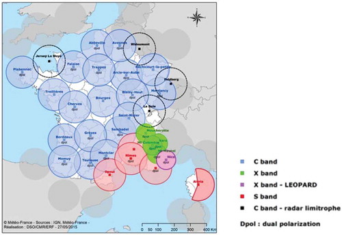
Figure 8. Cumulative rainfall depths by radar pixels over the sub-catchment area, for both C-band and X-band radar data for the three events studied.

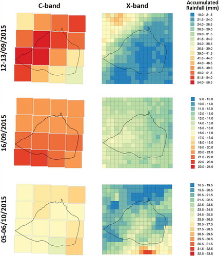
Figure 9. Time evolution of rain rate (top) and cumulative rainfall (bottom) over the whole sub-catchment area for the two data products (Météo-France C-band, in green; ENPC X-band, in blue) for the three events: 12–13 September 2015 (left), 16 September 2015 (centre) and 5–6 October 2015 (right).

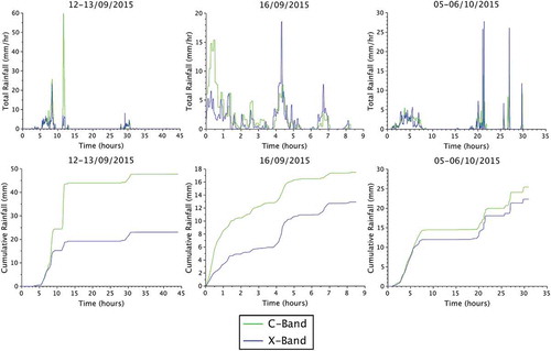
Figure 10. Comparison of water level obtained by simulations – using the calculated discharge coefficient and four variations (−50%, −25%, +25% and +50%) for the Cora basin – and measurements for the three events: (a) 12–13 September 2015, (b) 16 September 2015 and (c) 5–6 October 2015.

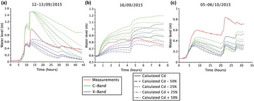
Figure 11. Time evolution of the difference in simulated water levels in Cora basin obtained with the highest (Cd + 50%) and the lowest (Cd − 50%) discharge coefficients used (top) and time evolution of the ratio of the same difference over the water levels in Cora basin obtained using the calculated Cd (bottom), for both radar data and for the three events studied: 12–13 September 2015 (left), 16 September 2015 (centre) and 5–6 October 2015 (right).

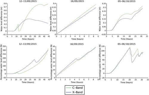
Figure 12. Comparison of water level in Cora basin obtained by simulations (using land use in the Massy area with priority and without priority order) and measurements for the three events: (a) 12–13 September 2015, (b) 16 September 2015 and (c) 5–6 October 2015.

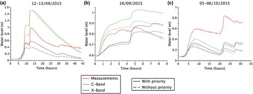
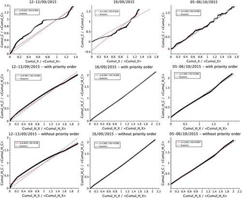
Figure 13. Relationships for cumulative total rainfall normalized by its mean (top), mean normalized cumulative water level using land use generated with priority order (centre), and mean normalized cumulative water level using land use generated without priority order (bottom), between C-band and X-band radars and three events: 12–13 September 2015 (left), 16 September 2015 (centre), 5–6 October 2015 (right). Continuous (red) line indicates the best linear fit, while the broken (blue) line corresponds to the first bisectrix.