Intensity–duration–frequency curves exploiting neighbouring extreme precipitation data

Figures & data

Table 1. Areas currently covered by different cities.

Location	Area (km^2)
Berlin	891
Hamburg	755
Munich	310
London	1572

Figure 1. Explanation of the methodology. D is the domain of interest, X is the centroid of D, S is the location of heaviest precipitation in D and G_i is the ith sub-area of D. For the temporal integral labels, we define Z_A,D as the averaged areal precipitation over D, Z_L as the precipitation at the centroid of D, Z_S,D as the heaviest precipitation in D and Z_G,D as the heaviest precipitation within the ith sub-area G_i. (See online version for colour versions of figures that are not colour in print.)

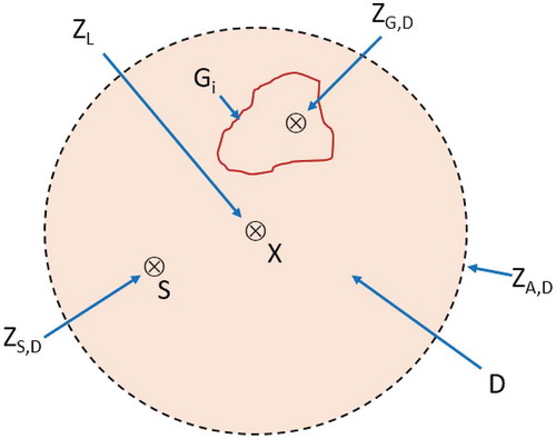
Figure 2. Pluviometer network of Reutlingen, Germany; the area is approximately 25 km square.

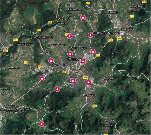
Figure 3. Distributions corresponding to the central four pluviometers in Figure 2 and the time aggregation of 1 h. Solid lines are the distributions of the individual stations, dashed lines are the distribution of the areal precipitation (green), the mean of the four distributions (blue), and the distribution of the maxima, Z_S,_D (red). The olive line shows the distribution of the maxima assuming that the stations are independent. The units on the horizontal axis are in mm and the vertical axis is cumulative probability.

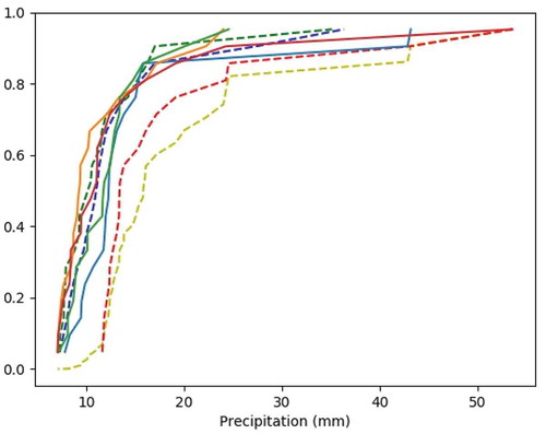
Figure 4. Distributions corresponding to the central eight pluviometers and the time aggregation of 1 h. See Figure 3 caption for explanation of lines and units.

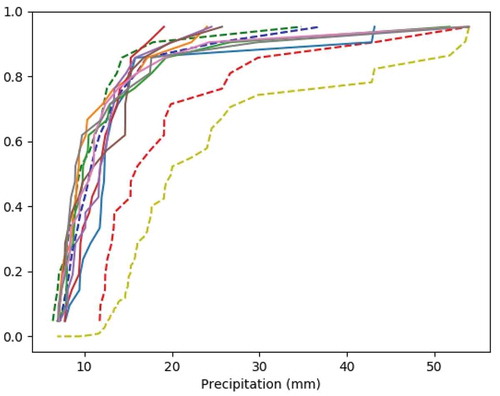
Figure 5. Distributions corresponding to the central four pluviometers and the time aggregation of 15 min. See Figure 3 caption for explanation of lines and units.

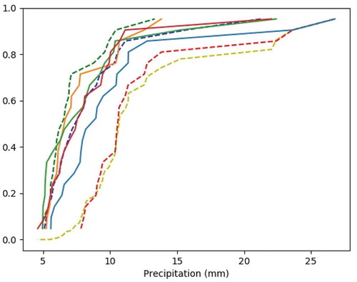
Figure 6. Distributions corresponding to the central eight pluviometers and the time aggregation of 15 min. See Figure 3 caption for explanation of lines and units.

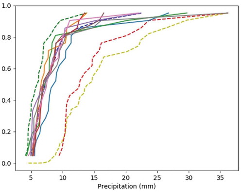
Figure 7. Distributions corresponding to the central four pluviometers and the time aggregation of 3 h. See Figure 3 caption for explanation of lines and units.

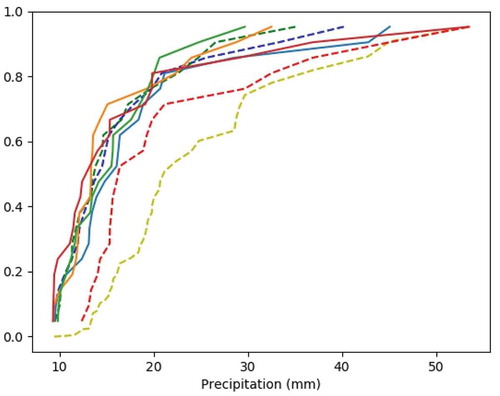
Figure 8. Distributions corresponding to the central eight pluviometers and the time aggregation of 3 h. See Figure 3 caption for explanation of lines and units.

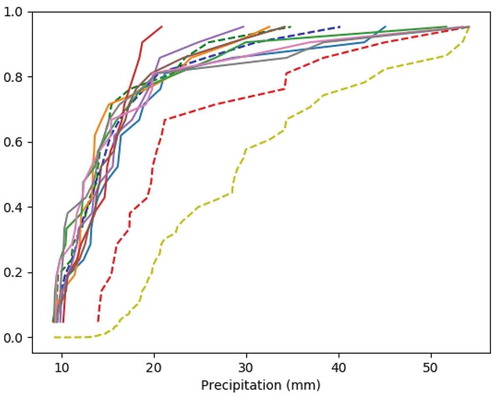
Figure 9. Configuration of the blocks considered (right). In the left figure the solid (red) line is the distribution of the maxima at the central point. The green dashed line is the distribution of the maxima of the single pixels (81 pixels each 500 m × 500 m) in the 4.5 km × 4.5 km square. The blue dashed line is the distribution of the maxima of the areal means calculated from the amounts in the nine squares (1.5 km × 1.5 km) each. Units are as in Figure 3 caption.

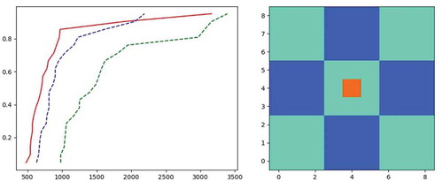
Figure 10. Stack algorithm used to simulate pseudo-random images from image scale statistics, from Clothier and Pegram (2002). WAR: wetted area ratio, IMF: image mean flux.

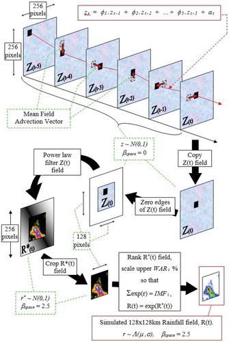
Figure 11. First, third and fifth top-ranked rainfall values of 5-min rainfall over 20 years in 1/10th mm in each 1 km² of 10 000 pixels (Z_L). The colour scale in all three panels ranges from 10 to 26 mm depth. The images in Figures 11–16 were derived from the SBM with Gaussian spatial dependence.

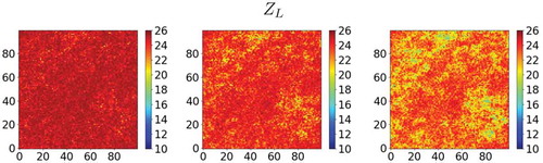
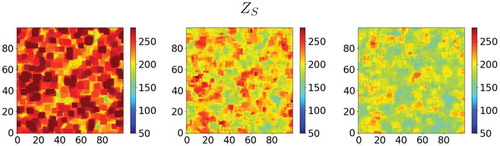
Figure 12. First, third and fifth top-ranked rainfall values of 60-min rainfall over 20 years in 1/10th mm in each 1 km² of 10 000 pixels (Z_L). The colour scale in all three panels ranges from 50 to 270 mm depth.

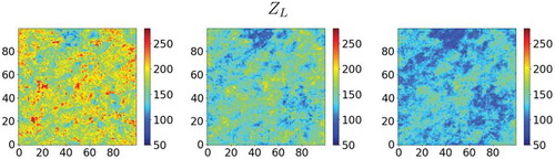
Figure 13. First, third and fifth top-ranked rainfall values of 60-min rainfall in each pixel for the case where we have selected nine pixels centred on the middle one (Z_S). The colour scale in all three panels ranges from 50 to 270 mm depth.

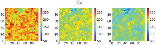
Figure 14. First, third and fifth top-ranked rainfall values of 60-min rainfall in each pixel for the case where we have selected 25 pixels centred on the middle one (Z_S). The colour scale in all three panels ranges from 50 to 270 mm depth.

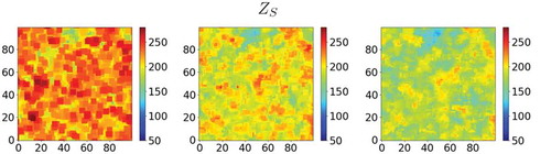
Figure 15. First, third and fifth top-ranked spatially averaged areal rainfall values of 60-min rainfall for the case where we have selected 25 pixels centred on the middle one (Z_A,_D). The maximum intensity of the averaged values is considerably lower than those in Figure 14. The colour scale in all three panels ranges from 50 to 270 mm depth.

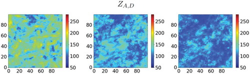
Figure 16. Distributions of extremes. Mauve: average of the single pixel extremes, orange: average of all the mean values over 3 × 3 blocks, blue: average of all the mean values over 5 × 5 blocks, red: average of the maxima over 3 × 3 blocks, and green: average of the maxima over 5 × 5 blocks.

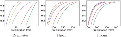
Figure 17. First, third and fifth top-ranked rainfall values (generated using χ² spatial copulas) of 60-min rainfall in each pixel for the case where we have selected 25 pixels centred on the middle one (Z_S). The colour scale in all three panels ranges from 50 to 270 mm depth to compare with Figure 14.

Clothier, A. and Pegram, G. (2002). Space-time modelling of rainfall using the string of beads model: integration of radar and raingauge data, WRC report No 1010/ 1/02[ISBN 1 86845 835 0], South Africa: Water Research Commission. doi:10.1044/1059-0889(2002/er01)

 Google Scholar