Knowable moments for high-order stochastic characterization and modelling of hydrological processes

Figures & data

Table 1. Illustration of the fact that raising to a power and adding converges fast to the maximum value.

Linear, p = 1	Pythagorean, p = 2	Cubic, p = 3	High order, p = 8
3 + 4 = 7	3^2 + 4^2 = 5^2	3^3 + 4^3 = 4.5^3	3^8 + 4^8 ≈ 4^8
3 + 4 + 12 = 19	3^2 + 4^2 + 12^2 = 13^2	3^3 + 4^3 + 12^3 = 12.2^3	3^8 + 4^8 + 12^8 ≈ 12^8

Figure 1. Illustration of the slow convergence of the sample estimate of the eighth noncentral moment to its true value, which is depicted as a thick horizontal line and corresponds to a lognormal distribution LN(0,1), where the process is an exponentiated Hurst-Kolmogorov process (Koutsoyiannis 2016) with Hurst parameter H = 0.9. (Left) The sample moments are estimated from a single simulation of that process with length 64 000, where parts of this time series with sample size n from 10 to 64 000 are used for the estimation. Subsetting of the time series to sample size n was done either from the beginning to the end (thicker lines) or from the end to the beginning (finer lines). Continuous lines in the two cases represent the eighth moment estimates, ${\sum }_{i=1}^n{x}_i^p/n$, and dashed lines represent maximum values, ${\left(\underset{1\le i\le n}{max}\left(x_i\right)\right)}^p/n$. (Right) Sampling distribution of the eighth moment estimator ${\displaystyle {\sum }_{i=1}^n{\underset{\_}{x}}_i^8}/n$ estimated from 1000 simulated series of length 1000 each and visualized by the 99% prediction limits (percentiles), the median and the average, plotted as ratios to the true value. Theoretically, the ratio should be 1, but it is smaller by many orders of magnitude, and the convergence to 1 is very slow. The ratio to ${\left(\underset{1\le i\le n}{max}\left(x_i\right)\right)}^8/n$, also plotted, is close to 1.

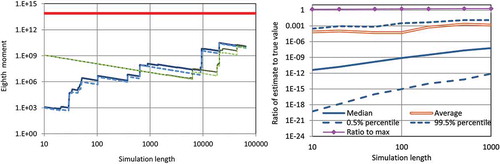
Figure 2. Illustration of agreement and disagreement of moment estimates with theoretical moments for normal distribution N(0,1) (left) and lognormal distribution LN(0,1) (right), where the K-moments correspond to q = 1 (upper row) and q = 2 (lower row). Note that, in the normal distribution, theoretical moments of odd order are zero (and thus not shown in the logarithmic plots) and that points corresponding to ${\mu }_p^{\prime }$ are (almost) indistinguishable from those corresponding to ${\mu }_p$. In the lognormal distribution the moments of odd order are depicted by the lower blue lines and series of points (circles), while the upper ones depict even moments.

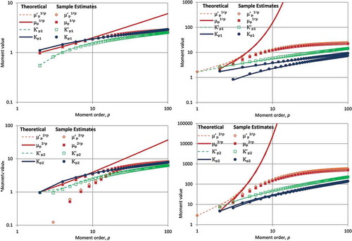
Figure 3. Illustration of the probability density function of: (upper) variability index ($K_{11}/K_{21}$, $\mu /\sigma \equiv K_{11}/\sqrt{K_{22}}$; note that the latter is the inverse of the common coefficient of variation); (middle), skewness index (${\mu }_3^{1/3}/\sigma$, $K_{31}/K_{21}$, $\mathrm{s}\mathrm{i}\mathrm{g}\mathrm{n}(K_{32})\sqrt{\left|K_{32}\right|/K_{22}}$); (lower) kurtosis index (${\mu }_4^{1/4}/\sigma ,$ ${\lambda }_4/{\lambda }_2$, $K_{41}/K_{21}$, $\sqrt{K_{42}/K_{22}}$). The panels of the left column correspond to the normal distribution Ν(0,1) and those of the right column to the lognormal distribution LN(0,2). The L-statistics, also plotted, differ from the K-statistics only for p = 4 (see Table 2). The densities are depicted after shifting to zero mean, while the bias (difference of the simulated mean from the theoretical value of Table 3, as a percentage of the latter) is also given in the legend of each panel.

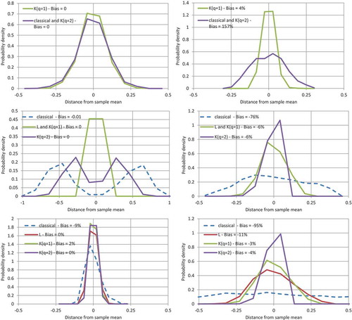
Figure 4. K-climacograms (left) and K-climacospectra (right) of turbulent velocity measured every 0.5 s, where the K-moments correspond to q = 1 (upper row) and q = 2 (lower row). Plot (2*) is constructed from the variance and (2**) corresponds to the standard deviation.

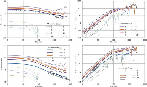
Figure 5. K-climacograms (left) and K-climacospectra (right) of rainfall rate for Iowa measured every 10 s, where the K-moments correspond to q = 1 (upper row) and q = 2 (lower row). Plot (2*) is constructed from the variance and (2**) corresponds to the standard deviation.

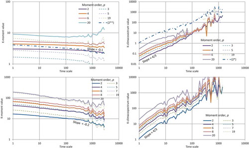
Figure 6. K-climacograms (left) and K-climacospectra (right) of daily rainfall at Padova, where the K-moments correspond to q = 2.

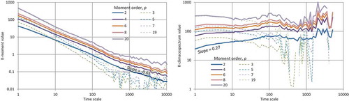
Figure 7. K-moments vs. moment order for: (upper left) turbulence velocity data; (upper right) synthetic data with same mean and variance as the turbulence data; (lower) daily rainfall data for Padova. Note that each curve is in fact a series of connected points whose shape is smooth by itself (not artificially smoothed).

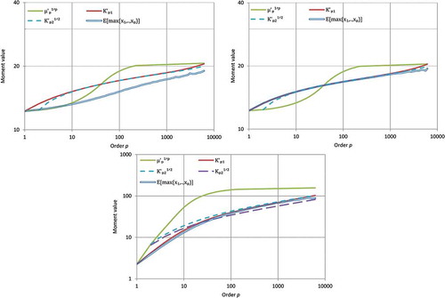
Table 2. Typical marginal statistical characteristics of distributions using different moment categories.

Characteristic	Order p	Option 1	Option 2	Option 3^a
Location	1	$K_{11}^{\prime }=\mu$ (the classical mean)
Variability	2	$K_{21}=2\left(K_{21}^{\prime }-\mu \right)=2{\lambda }_2$	$K_{22}={\mu }_2={\sigma }^2$(the classical variance)
Skewness (dimensionless)	3	$\frac{K_{31}}{K_{21}}=\frac{{\lambda }_3}{{\lambda }_2}$	$\frac{K_{32}}{K_{22}}$	$\frac{K_{33}}{K_{22}^{3/2}}=\frac{{\mu }_3}{{\sigma }^3}$
Kurtosis (dimensionless)	4	$\frac{K_{41}}{K_{21}}=\frac{4}{5}\frac{{\lambda }_4}{{\lambda }_2}+\frac{6}{5}$	$\frac{K_{42}}{K_{22}}$	$\frac{K_{44}}{K_{22}^2}=\frac{{\mu }_4}{{\sigma }^4}$

^aNot recommended for distribution fitting.

Table 3. Numerical illustration of the variation of typical marginal statistical characteristics for some customary distributions.

Characteristic	Variability		Skewness			Kurtosis
Distribution function^a	$K_{21}$ (1)^b	$K_{22}\left(2\right)$	$\frac{{\mathrm{K}}_{31}}{K_{21}}\left(1\right)$	$\frac{{\mathrm{K}}_{32}}{K_{22}}\left(2\right)$	$\frac{{\mathrm{K}}_{33}}{K_{22}^{3/2}}\left(3\right)$	$\frac{{\mathrm{K}}_{41}}{K_{21}}\left(1\right)$	$\frac{{\mathrm{K}}_{42}}{K_{22}}\left(2\right)$	$\frac{{\mathrm{K}}_{44}}{K_{22}^2}\left(3\right)$
U(0,1)	0.3333	0.08333	0	0	0	1.2	1.8	1.8
Ν(0,1)	1.128	1	0	0	0	1.465	2.103	3
LN(0,1/2)	0.6262	0.3647	0.2409	0.8146	1.750	1.335	2.239	8.898
LN(0,1)	1.716	4.671	0.4625	1.455	6.185	1.434	2.548	113.9
LN(0,2)	12.45	2926.4	0.7909	1.965	414.4	1.712	2.961	9.2 × 10^6
GP(1,1/6)	0.2181	0.06	0.4118	1.273	3.810	1.386	2.406	38.67
GP(1,1/4)	0.3810	0.2222	0.4545	1.429	7.071	1.418	2.522	∞
GP(1,1/3)	0.6	0.75	0.5	1.6	∞	1.455	2.657	∞

^aU: Uniform; N: Normal; LN: Lognormal; GP: Generalized Pareto with lower bound zero; the numbers in parentheses are the parameter values of the distributions.

^bThe numbers in parentheses refer to the Options defined in Table 2.

Koutsoyiannis, D., 2016. Generic and parsimonious stochastic modelling for hydrology and beyond. Hydrological Sciences Journal, 61 (2), 225–244. doi:10.1080/02626667.2015.1016950

 Web of Science ®Google Scholar