How much does an extreme rainfall event cost? Material damage and relationships between insurance, rainfall, land cover and urban flooding

Figures & data

Table 1. Statistical data of the municipalities in the LMA. Built-up areas (2007); buildings, dwellings and inhabitants (2011).

	Municipality	Area		Built-up areas		Buildings			Dwellings			Inhabitants
		(km^2)	(%)	(km^2)	(%)	(no.)	(no./km^2)	(%)	(no.)	(no./km^2)	(%)	(no.)	(no./km^2)	(%)
Northern LMA	Amadora	23.8	0.8	14.8	62.0	13 696	575.8	3.1	88 036	3701.4	5.9	175 136	7363.4	6.2
	Cascais	97.4	3.2	48.6	49.9	43 624	447.9	9.7	109 171	1120.8	7.3	206 479	2119.9	7.3
	Lisbon	84.9	2.8	61.6	72.5	52 496	618.0	11.7	323 981	3814.1	21.8	547 733	6448.2	19.4
	Loures	169.3	5.6	41.9	24.7	31 095	183.7	6.9	99 344	586.8	6.7	205 054	1211.2	7.3
	Mafra	291.7	9.7	41.9	14.4	28 002	96.0	6.2	42 957	147.3	2.9	76 685	262.9	2.7
	Odivelas	26.4	0.9	15.0	56.8	16 344	620.1	3.6	69 238	2626.9	4.7	144 549	5484.3	5.1
	Oeiras	45.9	1.5	26.2	57.1	18 243	397.6	4.1	86 162	1877.9	5.8	172 120	3751.3	6.1
	Sintra	319.2	10.6	84.3	26.4	56 903	178.3	12.7	182 854	572.8	12.3	377 835	1187.7	13.4
	Vila Franca de Xira	318.1	10.6	32.5	10.2	16 984	53.4	3.8	65 125	204.7	4.4	136 886	1066.4	4.9
Southern LMA	Alcochete	128.4	4.3	7.9	6.2	4 575	35.6	1.0	8 829	68.8	0.6	17 569	250.2	0.6
	Almada	70.2	2.3	32.4	46.2	34 163	486.6	7.6	101 536	1446.2	6.8	174 030	4782.3	6.2
	Barreiro	36.4	1.2	12.8	35.3	11 008	302.5	2.5	41 772	1147.9	2.8	78 764	246.7	2.8
	Moita	55.3	1.8	12.1	22.0	12 398	224.4	2.8	34 673	627.5	2.3	66 029	1194.9	2.3
	Montijo	348.6	11.6	21.1	6.1	12 996	37.3	2.9	26 766	76.8	1.8	51 222	146.9	1.8
	Palmela	465.1	15.5	39.9	8.6	21 631	46.5	4.8	33 196	71.4	2.2	62 831	135.1	2.2
	Seixal	95.5	3.2	38.7	40.5	30 124	315.4	6.7	79 552	833.0	5.3	158 269	1657.3	5.6
	Sesimbra	195.5	6.5	26.0	13.3	20 433	104.5	4.6	31 837	162.9	2.1	49 500	253.2	1.8
	Setúbal	230.3	7.7	37.3	16.2	24 242	105.3	5.4	62 829	272.8	4.2	121 185	526.2	4.3
Totals	Northern LMA	1376.7	45.9	366.8	26.6	277 387	201.5	61.8	1 066 868	775.0	71.7	2 042 477	1483.6	72.4
	Southern LMA	1625.2	54.1	228.4	14.1	171 570	105.6	38.2	420 990	259.0	28.3	779 399	479.6	27.6
	LMA	3001.9	100	595.2	19.8	448 957	149.6	100	1 487 858	495.6	100	2 821 876	940.0	100

Figure 1. Location of the study area, showing the raingauge locations and the municipalities of the Lisbon Municipal Area (LMA).

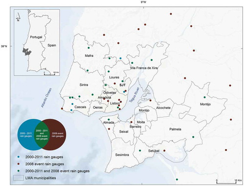
Table 2. Definitions of the concepts used in this research.

Concept	Definition
APS claim	Request to an insurance company made by a policyholder when flooding that affects the property occurs.
Capital sum affected	Amount of capital (€) insured in the insurance policy when an APS claim is reported.
Payouts	Amount of money (€) paid by an insurance company to a policyholder when an APS claim is reported. The maximum value is equal to the capital sum affected.

Figure 2. Large-scale atmospheric circulation and dynamic features of the extreme event of 18 February 2008: (a) 500 mb geopotential heights (dam), (b) sea-level pressure (mb), (c) total column water vapour (mm), (d) convective available potential energy (J kg⁻¹). All panels refer to 12:00 h UTC on 17 February 2008. Source of reanalysis data: www.ecmwf.int.

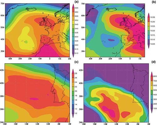
Figure 3. Spatial representation of the 24-h maximum rainfall during the 2008 event in the LMA.

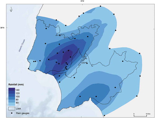
Figure 4. High-magnitude rainfall in the LMA at the São Julião do Tojal raingauge: (a) annual maximum daily rainfall for the period 1938/39–2011/12 and (b) IDF curves for several return periods and for the 1967, 1983 and 2008 rainfall events.

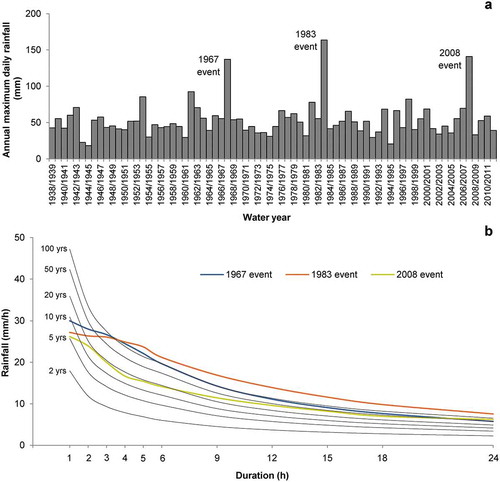
Figure 5. Temporal evolution of APS claims and payouts in the LMA (2000–2011): (a) number of APS claims and payouts, (b) accumulated APS claims and payouts.

Figure 6. Annual and monthly values of insurance data in the LMA (2000–2011) and the weight of the 2008 event: (a) number of APS claims per year, (b) payouts per year, (c) APS claims per month and (d) payouts per month. Note: the APS database ends in October 2011. This year only has records for 10 months; November and December values are therefore the result of accumulated values of only 11 years of records, unlike the other months (12 years).

Figure 7. Spatial distribution of the total APS claims (2000–2011) and those resulting from the 2008 event in the LMA.

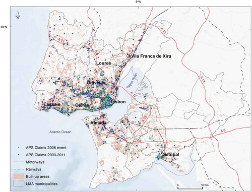
Figure 8. Rainfall vs APS claims for each APS event at 1, 3, 6, 12 and 24 hours on the SJT raingauge. Note: only the APS events with APS claims located within a 10 km radius of the SJT raingauge are represented.

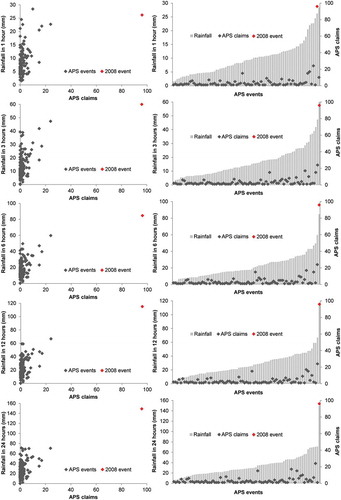
Figure 9. Temporal evolution of four rainfall events that caused a different number of APS claims in a 10 km radius of the SJT raingauge.

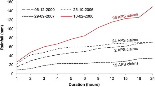
Figure 10. Likelihood levels of flooding for the SJT raingauge.

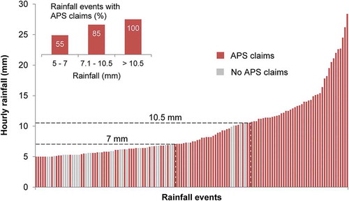
Table 3. Correlation matrix between land use/cover, building features and insurance data for the LMA municipalities. LIN: linear regression; LOG: logarithmic regression.

	Built-up areas (%)	Buildings/km^2	Dwellings/km^2	Insurance policies/km^2	APS claims/km^2	Capital sum affected/km^2	Payouts/km^2
Built-up areas (%)		0.97 (LIN)	0.92 (LIN)	0.95 (LOG)	0.94 (LOG)	0.85 (LOG)	0.88 (LOG)
Buildings/km^2	0.97 (LIN)		0.92 (LIN)	0.93 (LOG)	0.91 (LOG)	0.76 (LOG)	0.83 (LOG)
Dwellings/km^2	0.92 (LIN)	0.92 (LIN)		0.99 (LIN)	0.95 (LIN)	0.78 (LOG)	0.83 (LIN)
Insurance policies/km^2	0.95 (LOG)	0.93 (LOG)	0.99 (LIN)		0.94 (LIN)	0.79 (LOG)	0.83 (LIN)
APS claims/km^2	0.94 (LOG)	0.91 (LOG)	0.95 (LIN)	0.94 (LIN)		0.83 (LOG)	0.95 (LIN)
Capital sum affected/km^2	0.85 (LOG)	0.76 (LOG)	0.78 (LOG)	0.79 (LOG)	0.83 (LOG)		0.88 (LIN)
Payouts/km^2	0.88 (LOG)	0.83 (LOG)	0.83 (LIN)	0.83 (LIN)	0.95 (LIN)	0.88 (LIN)

Figure 11. Scatter chart between the APS claims per built-up km² and the maximum rainfall in 24 h for the 2008 event.

Figure 12. Material damage by type of flooding in the LMA and in the Lisbon municipality: (a) and (d) APS claims, (b) and (e) payouts, and (c) and (f) payouts per APS claim. (a), (b) and (c) correspond to the LMA, and (d), (e) and (f) to the Lisbon municipality.