Figures & data
Table 1. Rainfall and streamflow stations for each sub-catchment considered in the study. Australian Bureau of Meteorology station numbers are given in parentheses.
Figure 1. Study area and locations of the sub-catchments and rainfall and streamflow stations.
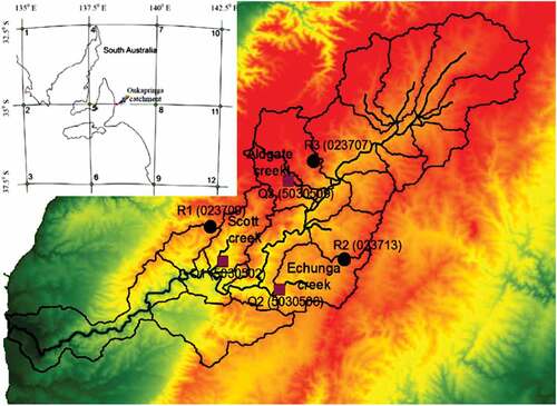
Figure 2. Mean and standard deviation of observed and simulated rainfall for different months of the year at three rainfall stations: from left to right, R1, R2 and R3, corresponding to the three study sub-catchments, for the validation periods (a) 1987–2000 and (b) 1981–2000. Solid curves represent the observations, while the box plots show the range of median and inter-quartile range (IQR) values for 1000 simulations. The whiskers represent 1.5 IQR from the box end.
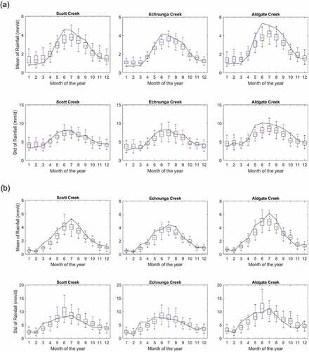
Table 2. Lags of statistically significant (at the 95% significance level) maximum correlation between decomposed rainfall sub-series and streamflow for three sub-catchments.
Figure 3. Decomposed sub-series (details, D1–D8 and approximation, A8) of the standardized rainfall series at rainfall station R1.
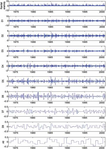
Table 3. Summary of fitted models for each sub-catchment with significant covariates for different parameters of the distribution.
Table 4. Comparison between the observed and median simulated daily streamflow for three sub-catchments over the calibration and validation periods. Avg: average streamflow (ML/d); SD: standard deviation of streamflow (ML/d); Max: maximum streamflow (ML/d); MB: mean bias; Scorr: Spearman correlation.
Figure 4. Scatterplots of observed and median simulated monthly streamflow for the calibration (left) and validation (right) periods.
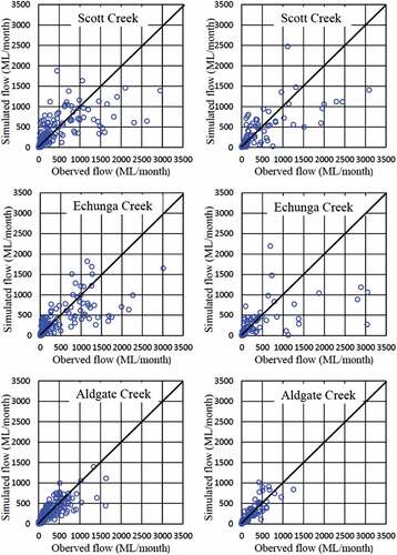
Table 5. Comparison between the observed and median simulated monthly streamflow for three sub-catchments over the calibration and validation periods. Avg: average of streamflow (ML/month); SD: standard deviation of steamflow (ML/month); CV: coefficient of variation; R2: coefficient of determination; NSE: Nash-Sutcliffe efficiency criterion.
Figure 5. Flow duration curves (FDC) of daily streamflow for the Scott Creek, Echunga Creek and Aldgate Creek sub-catchments. Blue and red curves represent the FDCs of the observed streamflow in the calibration (1973–1990) and validation (1991–2000) periods, respectively; grey curves represent the FDCs for individual simulations.
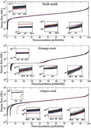
Figure 6. Scatterplots of observed and median simulated monthly streamflow for the calibration (left) and validation (right) periods using the model developed with historical RCAN.
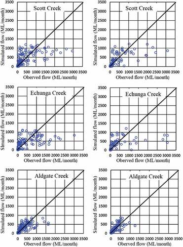
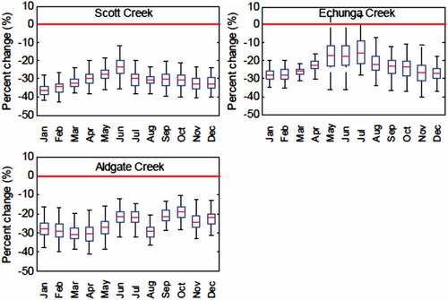
Figure 7. Projected changes (%) in streamflow for the CanESM2 GCM under the RCP4.5 scenario for the period 2041–2060 compared to the reference period 1973–2000. The boxplots depict the range of median and inter-quartile range (IQR) values for each model for 100 simulations; the whiskers represent 1.5 IQR from the box end.