Revealing hidden persistence in maximum rainfall records

Figures & data

Figure 1. Map of the 60 stations with longest records used in the analysis.

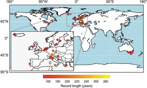
Figure 2. Explanatory graph of mathematical formulation: (a) Parent time series, (b) POT series, (c) temporal distribution of counts of POT at basic scale k = 1, (d) temporal distribution of counts of POT occurrences at scale k = 10 and (e) block maxima series at scale k = 10.

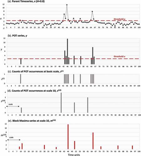
Table 1. Properties of the benchmark samples used in the experiments.

Distribution type	Parameters			Mean	Variance	Skewness	Kurtosis	H	Length
	Shape	Scale	Location
Normal	–	2.6	1.25	1.25	2.6	0	3	0.5–0.99	10^6
Gamma	0.1	5.1	-	0.51	2.6	6.325	63	0.5–0.99	10^6
Gamma	0.01	16.125	-	0.16	2.6	20	603	0.5–0.99	10^6
Pareto	0.1	1	0	1.11	1.54	2.81	17.83	0.5–0.99	10^6
Pareto	0.2	1	0	1.25	2.6	4.65	73.8	0.5–0.99	10^6

Figure 3. Visualization of three time series with H = 0.8 and different marginal distributions generated from the 4-moment SMA scheme (Dimitriadis and Koutsoyiannis 2018). The legends report, respectively, the mean, standard deviation, coefficient of skewness and coefficient of kurtosis of each distribution.

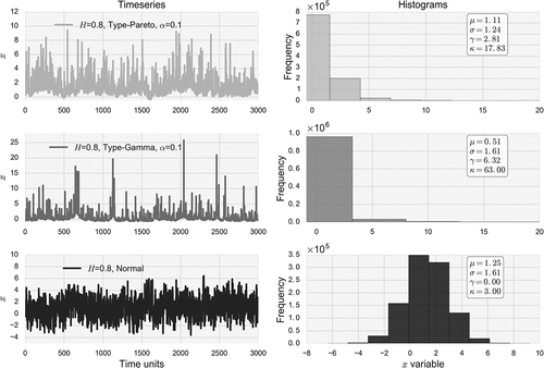
Figure 4. H parameters estimated from block maxima series at increasing scale of filtering for (a) benchmark series of length 10⁶ from HK models with H = 0.8 following normal and type-Pareto distributions, and (b) average H values from 10³ Monte Carlo simulations for HK models with H = 0.7 and three different marginal distributions, type-gamma, type-Pareto and normal.

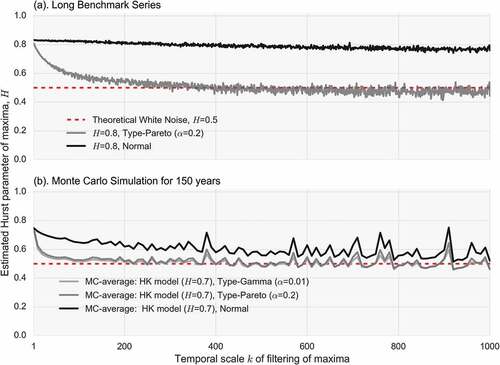
Figure 5. Index of dispersion of POT occurrences vs scale (double logarithmic axes) and estimated H parameters for scales > 500 for (a) benchmark series of length 10⁶ from HK models with theoretical H = 0.8 following normal and type-Pareto distributions, and (b) average values from 10³ Monte Carlo simulations for HK models with theoretical H = 0.7 and three different marginal distributions, type-gamma, type-Pareto and normal.

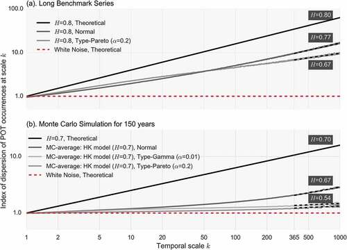
Figure 6. Minus natural logarithm of non-exceedence probability vs scale (NEPvS) index on double logarithmic axes along with the fit of the proposed model (Equation 2) for (a) benchmark non-Gaussian time series (type-gamma and type-Pareto), and (b) benchmark normal time series, for a range of H parameters.

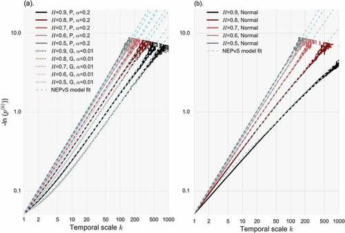
Figure 7. Minus natural logarithm of non-exceedence probability vs scale (NEPvS) index on double logarithmic axes for white-noise time series and two sample lengths: 150 × 365 and 300 × 365.

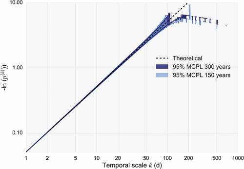
Figure 8. Minus natural logarithm of non-exceedence probability vs scale (NEPvS) index on double logarithmic axes for white-noise time series (length 150 × 365) and variations of the sampling threshold of extremes.

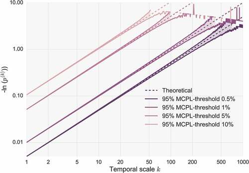
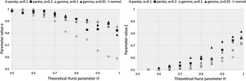
Figure 9. (a) Parameter η variation and (b) parameter ξ variation for increasing H parameter and different combinations of the sampling threshold and distribution type.

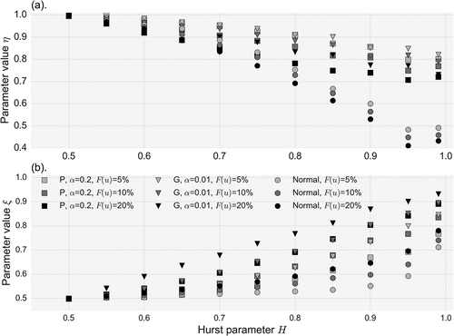
Figure 10. Minus natural logarithm of non-exceedence probability vs scale (NEPvS) index on double logarithmic axes along with 95% MCPL for (a) H = 0.7 with type-gamma (α = 0.1) and type-Pareto (α = 0.2) and white noise, and (b) H = 0.7 for two type-gamma distributions with α = 0.1 and α = 0.01.

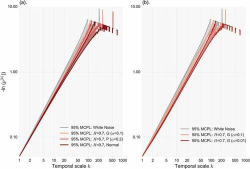
Figure 11. Minus natural logarithm of non-exceedence probability vs scale (NEPvS) index on double logarithmic axes for white-noise time series and seasonal and deseasonalized series by methods 1 (M1) and 2 (M2) for the stations of (a) Oxford, (b) Athens and (c) Helsinki.

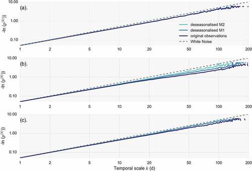
Table 2. Summary statistics (first and third quantiles, Q1 and Q3, mean and standard deviation, SD) of the properties of the rainfall dataset. Mean, variance, skewness and kurtosis are estimated for the wet record.

Statistic	Mean	Variance	Skewness	Kurtosis	Prob. dry	Hdaily	Hannual		Years	Missing %
Q1	3.68	24.85	2.9	17.28	0.47	0.56		0.55	153	0.75
Mean	4.98	64.85	3.39	24.03	0.55	0.63		0.67	169.25	2.62
Q3	5.91	64.64	3.54	25.85	0.61	0.7		0.77	173	1.31
SD	2.27	94.15	0.72	10.94	0.11	0.09		0.13	24.66	5.11

Figure 12. Empirical climacograms of the 60 daily rainfall series used in the analysis along with theoretical lines for H = 0.5, 0.6, 0.7, 0.8.

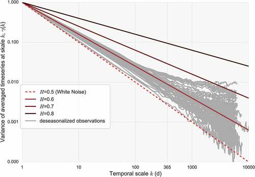
Figure 13. Minus natural logarithm of non-exceedence probability vs scale (NEPvS) index on double logarithmic axes for deseasonalized series for the 28 rainfall records in The Netherlands along with 95% MCPL of the fitted model with H = 0.7, for four different thresholds: (a) 10%, (b) 5%, (c) 1% and (d) 0.5%.

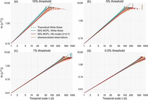
Figure 14. Minus natural logarithm of non-exceedence probability vs scale (NEPvS) index on double logarithmic axes for the deseasonalized series of Stykkisholmur, Iceland, along with 95% MCPL of the fitted models with H = 0.65 and H = 0.7, for four different thresholds: (a) 10%, (b) 5%, (c) 1% and (d) 0.5%.

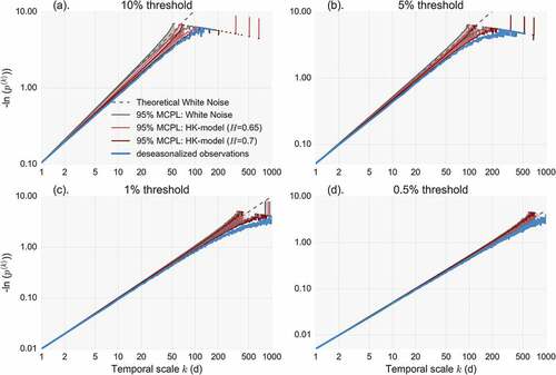
Figure 15. Boxplots of (a) parameter η, (b) parameter ξ and (c) RMSE from the fitting of the model to the seasonal and deseasonalized series by M1 for three different thresholds (1%, 5% and 10%).

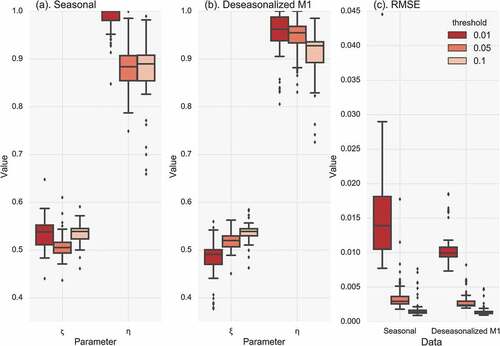
Figure A1. Plots of η and ξ parameters vs the H parameter and polynomial fitting for the distributions: (a) type-Pareto with α = 0.1, (b) type-Pareto with α = 0.2, (c) type-gamma with α = 0.1 and (d) type-gamma with α = 0.01.

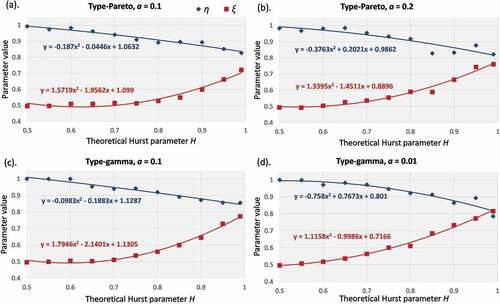
Figure A2. Plots of η and ξ parameters vs the H parameter and polynomial fitting for the normal distribution.

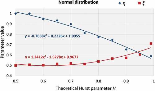
Figure A3. Plots of η and ξ parameters vs the H parameter for the distributions type-Pareto, with α = 0.1 and α = 0.2, type-gamma with α = 0.1 and α = 0.01 and normal.

Dimitriadis, P. and Koutsoyiannis, D., 2018. Stochastic synthesis approximating any process dependence and distribution. Stochastic Environmental Research and Risk Assessment, 32, 1493–1515. doi:10.1007/s00477-018-1540-2

 Web of Science ®Google Scholar