Figures & data
Figure 1. (a) Geographical location of Gharehsoo River Basin (GRB) in Iran; (b) geological map of the basin and Ardabil aquifer, (c) and geographical distribution of the selected piezometers on Ardabil aquifer.
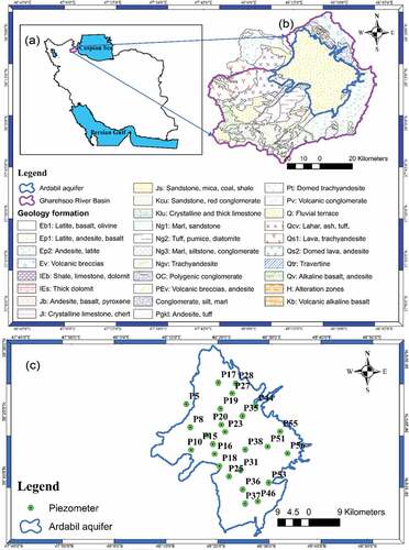
Table 1. Statistics of the piezometric stations with number and percentage of missing data for each piezometer, ordered from maximum to minimum.
Figure 2. Schematics of the distribution of multi-channel data for MSSA; t, x and s axes correspond to time-series length N, number of multi-channels L and number of lags M, respectively. There are special cases in MSSA, namely for L = 1, MSSA becomes SSA, and for M = 1, MSSA becomes conventional PCA (Myung Citation2009).
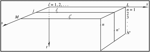
Figure 3. (a) Pearson cross-correlation matrix for all piezometric stations, with (b) significant levels. Note that N/D in the diagonals denotes that the autocorrelation significances has not been defined.
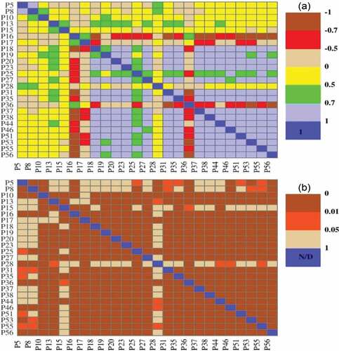
Figure 4. Histograms for the selected piezometers representing different types of probability distribution function (pdf) (see ).
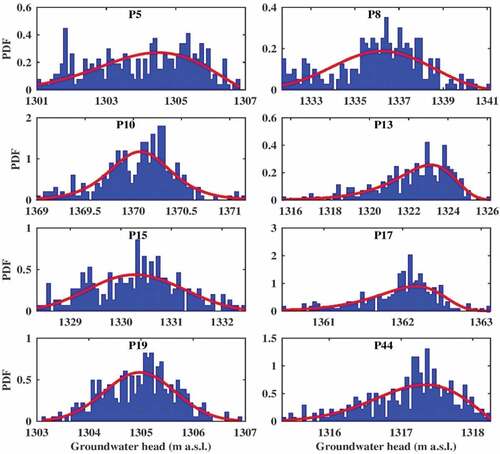
Table 2. The most suitable fitted probability distribution function, pdf (based on AIC) for each piezometer. GEV: generalized extreme value.
Figure 5. The selected window length, L (denoted by *) under SSA gap filling and reconstruction for P19 using objective function RMSE.
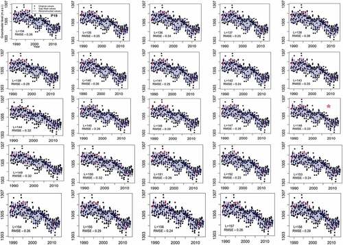
Figure 6. The selected window length, M (denoted by *) under MSSA gap filling and reconstruction for P19 using objective function RMSE.
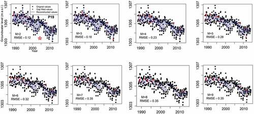
Figure 7. The selected window length, L (denoted by *) under SSA gap filling and reconstruction for P56 using objective function RMSE.
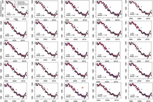
Figure 8. The selected window length, M (denoted by *) under MSSA gap filling and reconstruction for P56 using objective function RMSE.
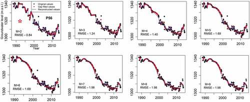
Figure 9. Original groundwater-level time series containing missing values represented by discontinuous time series in eight selected piezometric stations.
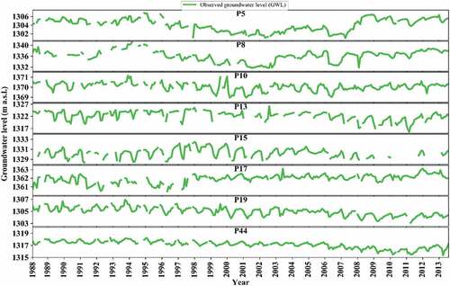
Table 3. Comparison of SSA and MSA in reconstruction of the groundwater-level time series for 25 piezometric stations.
Figure 10. Comparison of the reconstructed groundwater levels (GWL) and gap values filled using SSA and MSSA models for eight selected piezometers.
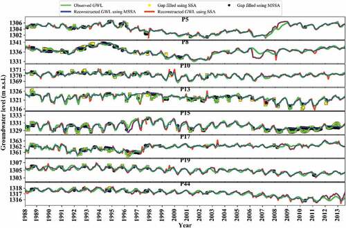
Figure 11. Reconstructed groundwater level using SSA and MSSA for 25 piezometric stations.
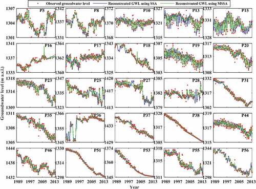
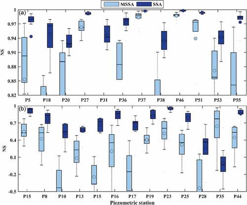
Figure 12. Box-and-whisker plots for the assessment of SSA and MSSA methods in terms of Nash-Sutcliffe efficiency (NS) for artificial gap values induced during cross-validation analysis for each piezometric station: (a) minimum and (b) maximum variability of NS in the piezometric stations.