
Figures & data
Figure 1. Structure of the basic auto-encoder.
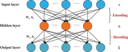
Figure 2. Structure of the ELM-CDAE.
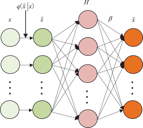
Figure 3. Structure of the proposed model (ELM-CDAE).
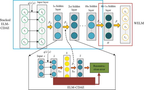
Figure 4. Distribution of the water quality monitoring stations in the study area.
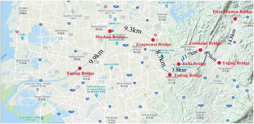
Table 1. Correlation coefficient of water temperature and electrical conductivity between different stations. #1 is the First Zengwen Bridge station and #8 is Xigang Bridge station (see ).
Table 2. Reference stations for different virtual stations in predicting water temperature and electrical conductivity.
Figure 5. Predictive effect of the model on water temperature at different depths: (a) station #1, (b) station #3, (c) station #5 and (d) station #7.
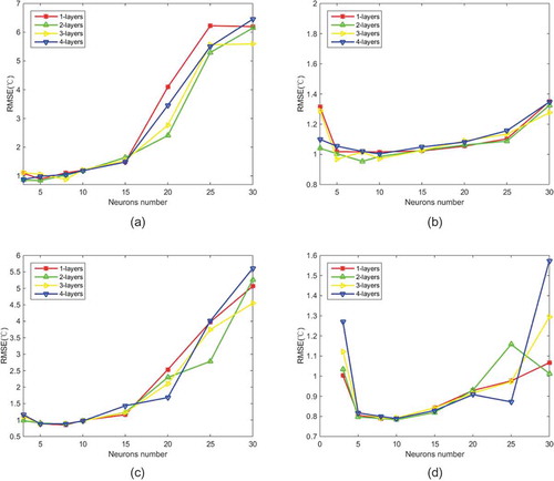
Figure 6. Predictive effect of the model on electrical conductivity at different depths: (a) station #1, (b) station #3, (c) station #5 and (d) station #7.
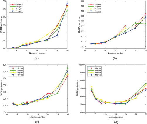
Figure 7. Prediction of water temperature for four virtual monitoring stations by different models: (a) station #1, (b) station #3, (c) station #5 and (d) station #7.
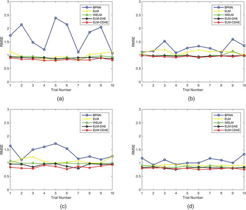
Figure 8. Predictions of electrical conductivity for four virtual monitoring stations by different models: (a) station #1, (b) station #3, (c) station #5 and (d) station #7.
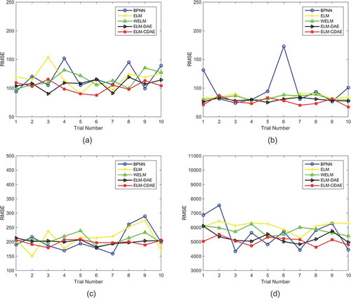
Table 3. Prediction results of different models for water temperature at different stations.
Table 4. Prediction results of different models for electrical conductivity at different stations.