Joint frequency analysis and uncertainty estimation of coupled rainfall–runoff series relying on historical and simulated data

Figures & data

Figure 1. Location of the study area.

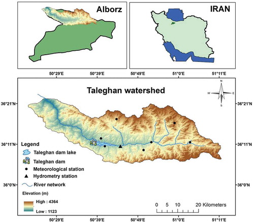
Figure 2. Spatial data used for HSPF model calibration: (a) hydrologic soil groups (HSG), (b) land-use map and (c) digital elevation model (DEM).

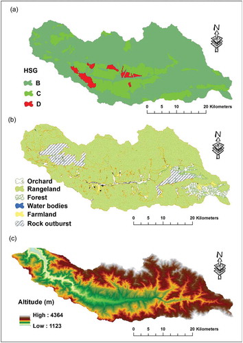
Figure 3. Design events estimation on quantile curves of p = 0.5 and p = 0.8.

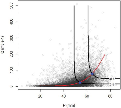
Figure 4. Flowchart of the study.

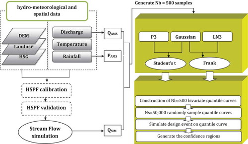
Figure 5. HSPF calibration before adjusting the KMELT parameter.

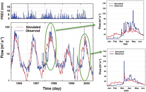
Table 1. The main parameters of the HSPF model calibrated for streamflow simulation. in: inch.

			Possible values
Parameter	Definition	Unit	Min	Max	Calibrated range
INFILT	Index to infiltration capacity	in/h	0.001	0.5	0.4
AGWRC	Base groundwater recession	none	0.85	0.999	0.971–0.996
LZSN	Lower zone nominal soil moisture storage	in	2	15	5–5.5
UZSN	Upper zone nominal soil moisture storage	in	0.05	2	1.12–2
DEEPFR	Fraction of groundwater inflow to deep recharge	none	0	0.5	0–0.01
INTFW	Interflow inflow parameter	none	1	10	1
IRC	Interflow recession parameter	none	0.3	0.85	0.3
BASETP	Fraction of remaining ET from baseflow	none	0	0.2	0–0.02
LZETP	Lower zone ET parameter	none	0.1	0.9	0.1–0.4
AGWETP	Fraction of remaining Et from active ground water	none	0	0.2	0.1
KMELT	Degree-day factor	in/d	0.14	0.2	0.14–0.2

Figure 6. (a) calibration (1995–2000) and (b) validation (2000–2005) of the HSPF model after adjusting the KMELT parameter.

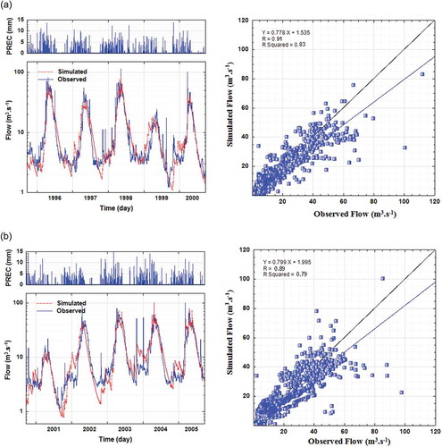
Table 2. HSPF model evaluation using the commonly used performance evaluation criteria.

	R^2	PBIAS (%)	ERMS (m^3 s^−1)	E
Calibration (1995–2000)
Daily	0.83	1.8	5.62	0.83
Monthly	0.87	5.99	4.62	0.86
Annual	0.84	1.8	1.77	0.83
Validation (2000–2005)
Daily	0.79	5.85	6.7	0.78
Monthly	0.86	9.49	5.2	0.85
Annual	0.91	5.84	2.9	0.81
Simulation (1979–2012)
Daily	0.71	15.3	8.3	0.66
Monthly	0.82	15.96	6.1	0.78
Annual	0.74	15.27	9.8	0.70

Table 3. Goodness-of-fit criteria for various univariate marginal distributions fitted to the selected data time series. AIC: Akaike Information Criterion; KS: Kolmogorov-Smirnov.

		KS
Data	Distribution family and estimated parameters	Statistic	p value	AIC
PAMS	Gaussian (γ = 0.88, μ = 49.56, σ = 12.32)	0.09	0.9	262
Qobs	P3 (α = 0.59, β = 41.9, γ = 3.48)	0.11	0.15	293
QSIM	LN3 (γ = 0.03, μ = 2.69, σ = 0.9)	0.08	0.95	269

Figure 7. Fitting univariate probability distributions to P_AMS, Q_obs and Q_SIM: (a), (c) and (e) cdf plots; and (b), (d) and (f) probability plots.

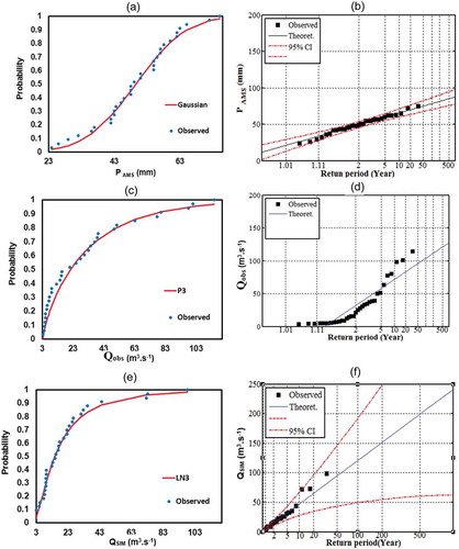
Table 4. Summary of copula goodness-of-fit test results for the Cramer-von Mises criterion (Sn), and associated p values calculated from a parametric bootstrap test (10,000 bootstrap samples). The best-fit copulas are indicated in bold.

Data	Copula family	Sn	p-value	Estimated parameter	AIC
PAMS-Qobs	Student’s t	0.04	0.84	0.46 1.72	–8.71
	Clayton	0.05	0.84	0.88	–8.35
	Plackett	0.04	0.86	4.14	–8.37
	Gumbel	0.05	0.84	1.44	–5.21
	Frank	0.04	0.85	2.96	–7.50
	Gaussian	0.05	0.84	0.46	–5.80
PAMS-QSIM	Student’s t	0.16	0.12	0.33 30	–3.67
	Clayton	0.04	0.15	0.66	–4.08
	Plackett	0.03	0.36	3.42	–4.60
	Gumbel	0.06	0.11	1.16	–1.65
	Frank	0.03	0.27	2.55	–4.87
	Gaussian	0.04	0.08	0.39	–3.76

Figure 8. Joint probability and return periods (RT) of P_AMS-Q_obs and P_AMS-Q_SIM: (a) and (c) joint probability plots; and (b) and (d): RT plots.

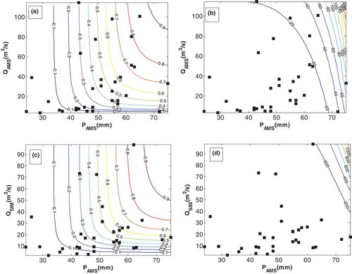
Figure 9. Conditional RT of (a) Q_obs given P_AMS, (b) Q_SIM given P_AMS.

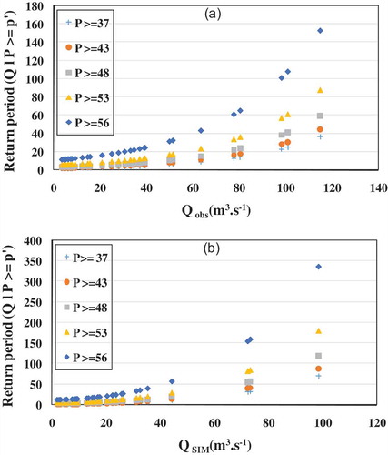
Figure 10. Uncertainty estimation of bivariate quantiles of P_AMS-Q_SIM at different probability levels of p = 0.5–0.99.

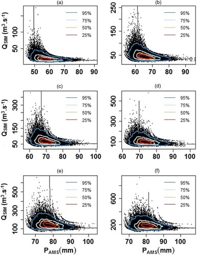
Figure 11. Uncertainty estimation of bivariate quantiles of P_AMS-Q_obs at different probability levels of p = 0.5–0.99.

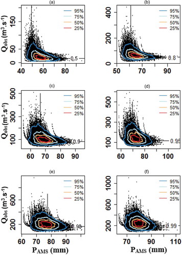
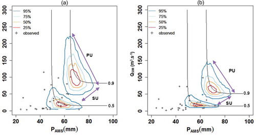
Figure 12. Comparison of uncertainties between (a) historical data and (b) HSPF simulation.