Seasonal patterns of suspended sediment load and erosion-transport assessment in a Mediterranean basin

Figures & data

Figure 1. General location of the study area. Isser Dam and meteorological stations (Chouly, code: 160601; Meurbah, code: 160602; Ouled Mimoun, code: 160607; Sidi Bounakhla, code: 160610), are represented by (black) squares and (blue) triangles, respectively. The gauge station of Sidi Abdelli (code: 160604) is represented by a (black) dot.

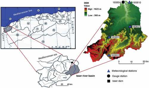
Table 1. Statistical values of the measured variables for the period 1988–2004. P: annual precipitation; SSC: suspended sediment concentration, Q_s: sediment flow; Q: runoff. SD: standard deviation.

	P (mm) (annual)	SSC (g/l) (daily)	$Q_s$(kg/s) (daily)	$Q\left({\mathrm{m}}^3/\mathrm{s}\right)$(avg. daily)	Consecutive days without SSC and Q measurements
Mean	322.93	0.97	13.92	1.22	3.13
SD	61.23	5.16	164.24	9.33	10.87
Min	269.94	0.01	0.0001	0.004	1.00
Max	409.71	67.20	3782.43	295.40	197.00

Figure 2. Available data for the study site. (a) Precipitation at four meteorological stations used as criteria for event selection and uncertainty analysis. (b) Flow measurements at the gauge station Sidi Abdelli. (c) Concentration and (d) sediment flow measured at the gauge station, and (e) periods without $\mathrm{S}\mathrm{S}\mathrm{C}$ and $Q$ data.

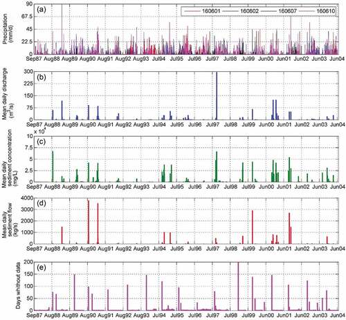
Figure 3. Flowchart illustrating the methodology developed for this work. Event-scale and continuous approaches are distinguished in order to assess seasonal SSY, SDR and basin–river interactions at the study site.

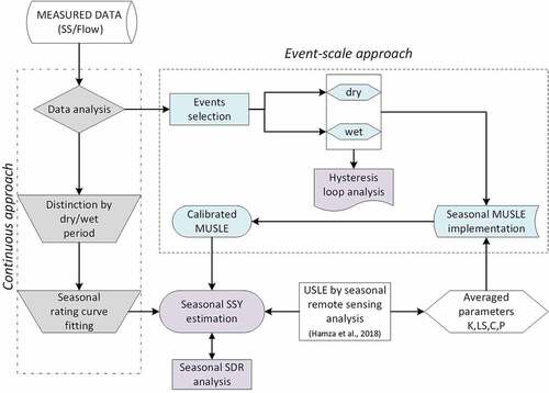
Figure 4. Accumulated rainfall with respect to the number of periods without SSC and $Q$ measurements for different time windows: (a) 3–5 days, (b) 3–50 days and 3–200 days.

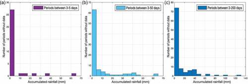
Figure 5. Relationship between SSC and water discharge from measured samples for (a) the whole period, and for (b) dry and (c) wet periods. The adjustment based on the $\mathrm{S}\mathrm{S}\mathrm{C}=\alpha Q^{\beta }$ relationship, with fitted parameters and the coefficient of determination. (d) Comparison with other Mediterranean environments is shown based on the following sources: Arbucies River: .Batalla and Sala (1994); Anoia River: Farguell and Sala (2006); Celone River: De Girolamo et al. (2015); Asser River: Mano et al. (2009); Mellah River: Khanchoul et al. (2009); Mellegue River: Selmi and Khanchoul (2016); and Eshtemoa River: Alexandrov et al. (2007).

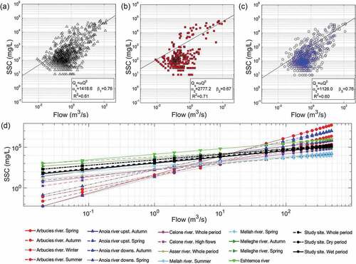
Figure 6. (a) Cumulative water discharge and sediment flow from measurements and rating curve estimations. Pulses of significant events and their impacts on sediment transport are clearly identified. (b) Resulting values of SSY obtained by considering increasing time windows without SSC and $Q$ measurements, assuming stationary conditions of flow.

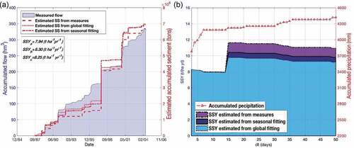
Figure 7. Distributed values of SDR, obtained by implementing the methodology of Borselli et al. (2008), and associated histograms for: (a)–(b) wet and (c)–(d) dry seasons.

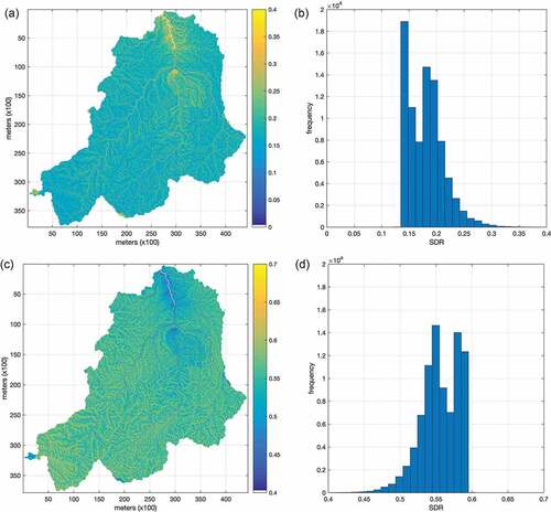
Table 2. Summary of seasons and hysteresis loop sense for the events selected. Shaded areas indicate the dry period and unshaded the wet period. The symbols and indicate clockwise and counter-clockwise direction, respectively.

Month	12	1	2	3	4	5	6	7	8	9	10	11
	Winter			Spring			Summer			Autumn
1
2
3
4
5
6
7
8
9
10
11
12

Figure 8. Hysteresis curves for the 12 largest events for which data were available in the historical data. D and W refer to dry and wet periods, respectively. Dots mark the loop direction (from dark blue to yellow).

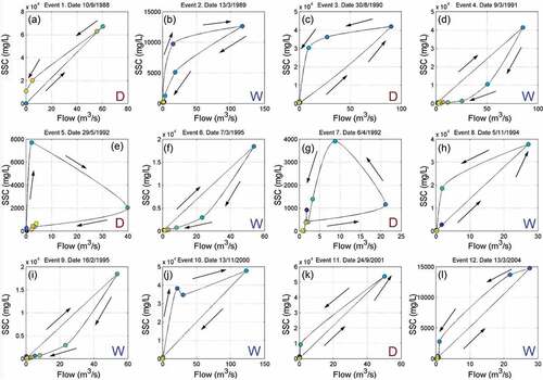
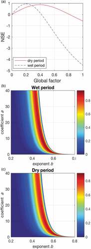
Table 3. Results of the MUSLE model parameters calibrated at the study area, a and b, and the global factor, $F_M$ for wet and dry periods. NSE: Nash–Sutcliffe efficiency criterion.

		$a$	$b$	$F_M$	NSE
Wet period	MUSLE original optimized	11.8	0.56	0.20	0.95
	MUSLE optimized	0.43	0.64	1	0.95
Dry period	MUSLE original optimized	11.8	0.56	0.39	0.87
	MUSLE optimized	0.05	0.79	1	0.91

Figure 9. Relationship between the estimated contribution of sediment measured for each event and that estimated with the MUSLE model for wet (blue triangle) and dry (red dot) periods.

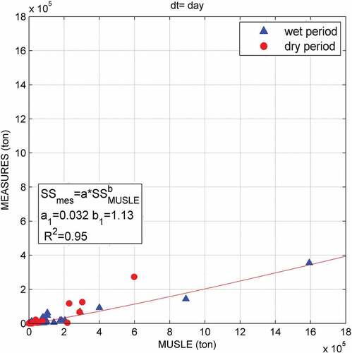
Figure 10. (a) Performance measured by NSE values of the global factor of MUSLE correction, $F_M$, for wet and dry periods. (b) Wet period and (c) dry period NSE values for the coefficient a and exponent b of the MUSLE model regionalized for the study area.

Batalla, R.J. and Sala, M. 1994. Temporal variability of suspended sediment transport in a Mediterranean sandy gravel-bed river. In: L.J. Olive, R.J. Loughran, and J.A. Kesby, eds. Variability in stream erosion and sediment transport (Proceedings of the Canberra symposium, December 1994). Wallingford, UK: International Association of Hydrological Sciences, IAHS Publ. no. 224, 299–306. https://iahs.info/uploads/dms/iahs_224_0299.pdf [Accessed 11 January 2020].

 Google Scholar

Farguell, J. and Sala, M., 2006. Seasonal trends of suspended sediment concentration in a Mediterranean basin (Anoia river, NE Spain). In: P.N. Owens and A.J. Collins, eds. Soil erosion and sediment redistribution in river catchments: measurement, modelling and management. Cranfield, 85.

 Google Scholar

De Girolamo, A.M., Pappagallo, G., and Porto, A.L., 2015. Temporal variability of suspended sediment transport and rating curves in a Mediterranean river basin: the Celone (SE Italy). Catena, 128, 135–143. doi:10.1016/j.catena.2014.09.020.

 Web of Science ®Google Scholar

Mano, V., et al., 2009. Assessment of suspended sediment transport in four alpine watersheds (France): influence of the climatic regime. Hydrological Processes, 23 (5), 777–792. doi:10.1002/hyp.v23:5.

 Web of Science ®Google Scholar

Khanchoul, K., Altschul, R., and Assassi, F., 2009. Estimating suspended sediment yield, sedimentation controls and impacts in the Mellah Catchment of Northern Algeria. Arabian Journal of Geosciences, 2 (3), 257–271. doi:10.1007/s12517-009-0040-6.

 Web of Science ®Google Scholar

Selmi, K. and Khanchoul, K., 2016. Sediment load estimation in the Mellegue catchment, Algeria. Journal of Water and Land Development, 31 (1), 129–137. doi:10.1515/jwld-2016-0044.

 Google Scholar

Alexandrov, Y., Laronne, J.B., and Reid, I., 2007. Intra-event and inter-seasonal behaviour of suspended sediment in flash floods of the semi-arid northern Negev, Israel. Geomorphology, 85 (1–2), 85–97. doi:10.1016/j.geomorph.2006.03.013.

 Web of Science ®Google Scholar

Borselli, L., Cassi, P., and Torri, D., 2008. Prolegomena to sediment and flow connectivity in the landscape: a GIS and field numerical assessment. Catena, 75 (3), 268–277. doi:10.1016/j.catena.2008.07.006.

 Web of Science ®Google Scholar