Water management for irrigation, crop yield and social attitudes: a socio-agricultural agent-based model to explore a collective action problem

Figures & data

Figure 1. Schematic representation of the system modelled. The farmed land (top) sits on the aquifer A and is divided into patches (squares), each representing a farm. The farmers (one for patch) are the agents, making strategic decisions relative to their farm. Farms are of the same size (A_farm), but the cultivated area can differ from farm to farm, depending on whether the farmer has invested in an on-farm pond or not. Two farms with contrasting features are presented on the right. In farm j, the farmer is short-view oriented (${\tau }_j<0.5)$, hence relies only on groundwater for irrigation and can cultivate the entire farm. In farm k, the farmer is long-view oriented (${\tau }_k>0$.5), hence invested in an on-farm pond (blue square), which occupies a part of the farm, thus reducing the cultivated area A_c,k.

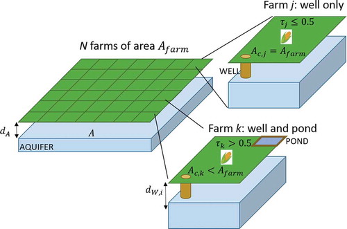
Figure 2. The farmer’s decision-making process for the irrigation source. The farmer’s attitude parameter ${\tau }_i$ is compared with a threshold: when ${\tau }_i$ > 0.5, the farmer is considered long-view-oriented and aims to rely also on the on-farm pond for irrigation; otherwise, the farmer is considered short-view-oriented and willing to rely only on groundwater for irrigation.

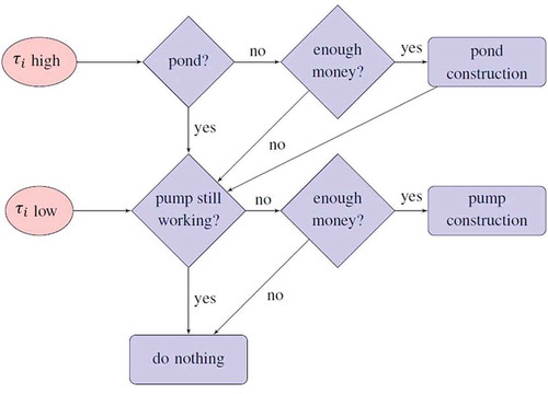
Figure 3. Temporal evolution of final crop biomass, water table and well depths in a 20-year sample model run, for four communities differing in their SOF-ratio. Dashed red lines refer to crop-biomass achieved by a short-view-oriented farmer, solid green lines to that achieved by a long-view-oriented farmer; in blue the depth of the water table and in purple the average depth of the wells. For enhanced visibility of the differences across communities and farmers, here the climatic conditions correspond to the extreme climate scenario, but similar patterns emerge also for more moderate scenarios. The farmers’ attitude does not evolve in time (i.e. $\mu =0$).

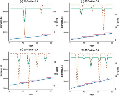
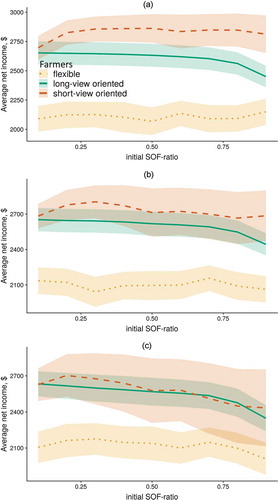
Figure 4. Average net economic gains over 30 years for long-view-(green solid line) and short-view-(red dashed line) oriented farmers, as a function of the SOF-ratio, under three different climate scenarios: a) current, b) intermediate, and c)extreme climate. Shaded areas extend over the average plus and minus the standard deviation. The farmers’ attitude does not evolve in time (i.e. $\mu =0$).

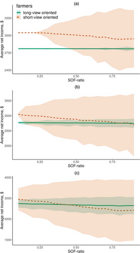
Figure 5. Water table depths, averaged over 100 simulations, in communities differing in SOF-ratio after 10 (circles) and 20 (triangles) years, with a starting water table depth of 5 m: (a) current climate, (b) intermediate climate and (c) drier climate. The farmers’ attitude does not evolve in time (i.e. $\mu =0$).

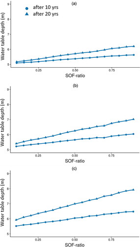
Figure 6. Average net economic gain over a period of 30 years in different communities, for the three climate scenarios: (a) current, (b) intermediate and (c) extreme climate. The shaded areas extend over the average plus and minus standard deviation for each curve. The farmers’ attitude does not evolve in time (i.e. $\mu =0$).

Figure 7. Average net economic gain over a period of 30 years within the different communities, for different initial depths of the groundwater (from 1 to 15 m, in steps of 1 m), for (a) current, (b) intermediate and (c) extreme climate scenario. The farmers’ attitude does not evolve in time (i.e. $\mu =0$).

Figure 8. Proportion of long-view-oriented, short-view-oriented and flexible farmers (i.e. farmers who changed their behaviour at least once during the period considered) after 30 years, as a function of the initial SOF-ratio, under the three climate scenarios: (a) current, (b) intermediate and (c) extreme). The memory decay rate is $\mu =2$. The values are averages over 100 simulations.

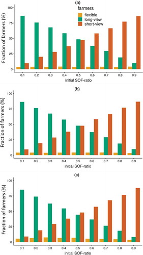
Figure 9. Average net economic gain over a period of 30 years for long-view-oriented farmers (solid green lines), short-view-oriented farmers (dashed red lines) and flexible farmers (i.e. farmers who changed their behaviour at least once; dotted yellow lines), under the three climate scenarios: (a) current, (b) intermediate and (c) extreme. Shaded areas extend over the average plus and minus the standard deviation of each curve. The memory decay rate is $\mu =\mathrm{0.2.}$.