Comparative analysis of scalar upper tail indicators

Figures & data

Figure 1. Schematic representation of Lorenz curves of three distributions with different Lorenz asymmetry coefficients.

Table 1. Parameter choices for the analysis of key properties. For all analyses, the shape parameter ξ of the GEV was predefined as -0.5, -0.25, 0, 0.25 and 0.5. This range is expected to envelope the range that is typically found in hydro-meteorological time series (e.g. Papalexiou and Koutsoyiannis 2013). Single values mark constant ones and several values indicate the variation of the parameter. For the analysis of scale invariance, location and scale parameters were paired, so that the ratio of µ and σ was kept equal to 2.5.

	Parameter
Focus of analysis	Scale parameter, σ	Location parameter, μ	Sample size, n
Sample size	16	40	25, 50, 75, 100, 150
Location shift	16	20, 40, 80, 200	100
Scale invariance	16, 32, 80	40, 80, 200	100

Table 2. Parameter ranges for the surprise analysis, showing the ranges of the randomly sampled three parameters of the GEV distribution and two parameters of the lognormal distribution. The ratio of scale and location (σ/µ) is varied accordingly. For the lognormal distribution the ratio is given by $\frac{\sigma }{\mu }=\sqrt{{\mathrm{e}}^{{\sigma }_L^2}-1}$ (e.g. Canchola 2018) and, thus, it is only dependent on the scale parameter of the lognormal distribution.

	Parameter range
Distribution	Shape parameter, ξ	Scale parameter, σGEV	Location parameter, μGEV	σ/μ
GEV	0 to 1	1 to 15	2 to 40	0.03 to 1
Lognormal		Scale parameter, σL	Location parameter, μL	σ/μ
		0.1 to 5	1 to 4	0.11 to 262,425

Figure 2. Boxplots of upper tail indicators for synthetic sampling distributions as a function of the parent shape parameter and sample size. Note that the y axis of the UTR is cut at the 90th percentile due to large outliers. For all boxplot graphics shown, the hinges represent the first and third quartiles, while the upper and lower whiskers represent the distance of 1.5 times the inter-quartile range from the upper and lower hinge, respectively.

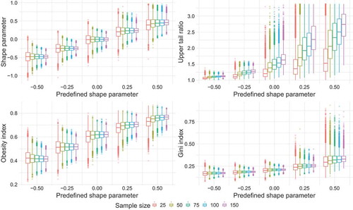
Figure 3. Boxplots of upper tail indicators for synthetic sampling distributions with sample size of 100, varying location parameter (20, 40, 80 and 200) and a constant scale parameter of 16.

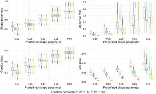
Figure 4. Boxplots of upper tail indicators for synthetic sampling distributions with sample size of 100, varying location parameter (20, 40 and 200) and constant σ/µ ratio.

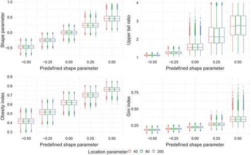
Figure 5. Scatter plots of upper tail indicator vs surprise factor for 10³ synthetic “true” distributions drawn from parent lognormal distributions. Each of the 10⁴ sampling distributions from the “true” distribution contains 50 values and the surprise factor is estimated for a 50-year event with α = 1.5.

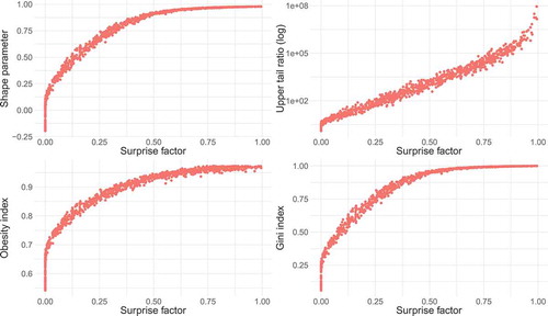
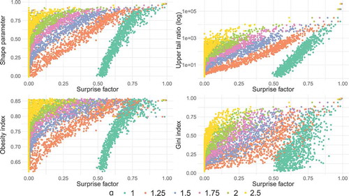
Figure 6. Scatter plots of upper tail indicator vs surprise factor f or 10³ synthetic “true” distributions drawn from parent GEV distributions. Each of the 10⁴ sampling distributions from the “true” distribution contains 50 values and the surprise factor is estimated for a 50-year event with α = 1.5.

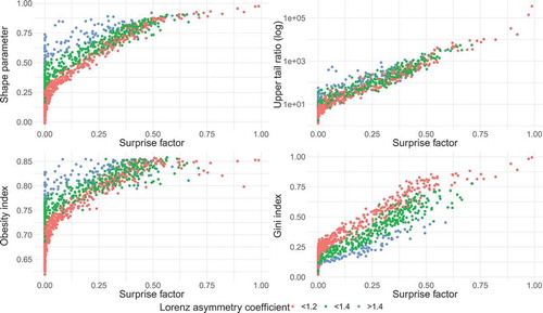
Figure 7. Upper tail indicators, surprise factor and Lorenz asymmetry coefficient of the synthetic “true” distributions plotted in the Lorenz space. Each point represents the point of maximum distance to the line of equality (inflection point of the Lorenz curve) of one GEV distribution and is coloured according to the selected parameter in the respective legend. The division into classes of the Lorenz asymmetry coefficient is illustrated on the bottom right.

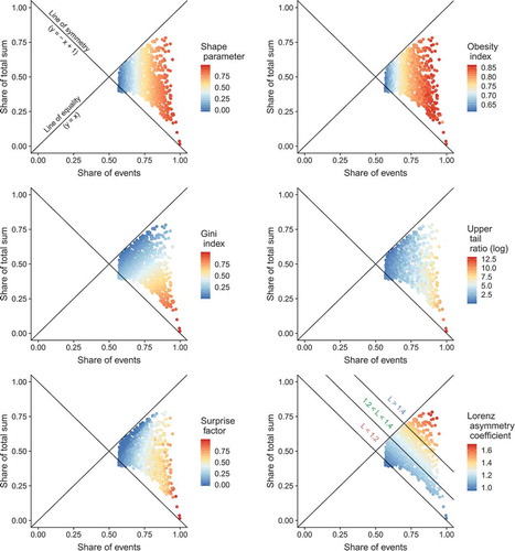
Table 3. Characteristics of the three example distributions of Fig. 8.

Parameter	Lognormal (orange)	GEV (red)	GEV (blue)
Shape parameter	0.63	0.61	0.62
Obesity index	0.85	0.79	0.81
Gini index	0.70	0.48	0.09
Upper tail ratio	43	168	20
Surprise factor (α = 1.5)	0.22	0.31	0.00
L	1.00	1.18	1.49
$X_{50\mathrm{y}\mathrm{r}}^{\mathrm{t}\mathrm{r}\mathrm{u}\mathrm{e}}$	367	235	39
σ	155.9^a	13	1
μ	57.8^a	26	22
σ/μ	2.70^a	0.50	0.05

^aFor the lognormal distribution, standard deviation, mean and coefficient of variation are given.

Figure 8. Three example distributions: density plots with log-scaled x axis (left) and the corresponding Lorenz curves (right).

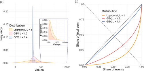
Figure 9. GEV-based surprise analysis with different degrees of surprise α.

Papalexiou, S.M. and Koutsoyiannis, D., 2013. Battle of extreme value distributions: A global survey on extreme daily rainfall. Water Resources Research, 49 (1), 187–201. doi:10.1029/2012WR012557

 Web of Science ®Google Scholar

Canchola, J.A., 2018. Correct use of percent coefficient of variation (%CV) formula for log-transformed data. MOJ Proteomics & Bioinformatics, 6 (3), 316–317.

 Google Scholar