Figures & data
Figure 1. Area of study and stations used (circles: Neuquen River basin; triangles: Limay River Basin).
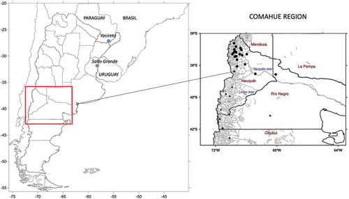
Figure 2. Evolution of the precipitation index, IE, used to represent the annual precipitation averaged over the Neuquen and Limay river basins.
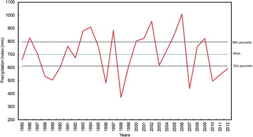
Figure 3. Mean monthly precipitation (mm) in the Limay (dashed line) and Neuquen (solid line) river basins.
Table 1. Definition of predictors defined considering the areas with significant (95%) IE difference between wet and dry years ( and ), averaged in DJF or MAM. The correlation between annual precipitation and the predictor is detailed in the last column. SST: sea-surface temperature; G500: geopotential height at 500 hPa.
Figure 4. Difference between wet and dry years for (a) SST, (b and c) G500, (d) U, (e) V and (f) PW composites in DJF prior to predicted winter precipitation.
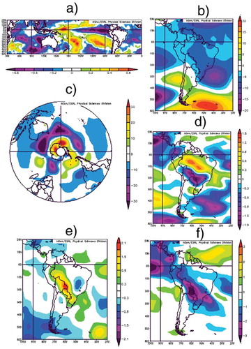
Figure 5. Difference between wet and dry years for (a) SST, (b and c) G500, (d) U, (e) V and (f) PW composites in MAM prior to predicted winter precipitation.
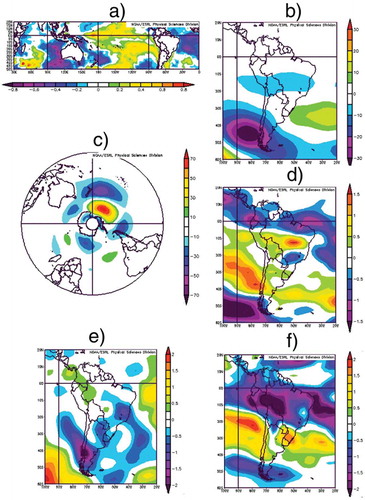
Table 2. Sets of independent potential predictors that are input into the models, the best model built for each set of predictors and the measure of accuracy given by CVI, AIC and AdjR2 coefficients.
Table 3. Percentage of cases correctly classified by each set of independent potential predictors that differ in one category and those wrongly classified as above-normal, normal or below-normal using the different models.
Figure 6. Observed and forecasted IE (mm) using the best model derived from Set 2 (see ). The prediction can be done in early March.
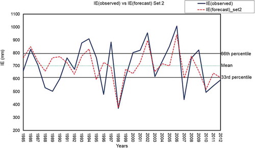
Table 4. Probability of detection (POD), false alarm ratio (FAR) and hit rate (H) for above-normal and below-normal cases derived using the different models. Best scores are indicated in bold.
Figure 7. Observed and forecasted IE (mm) using the best model derived from sets 1, 3 4 and 5 (). The prediction can be done in early June.
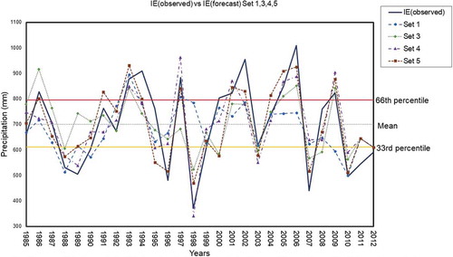
Figure 8. Forecast results for the period 2013–2017 (top) and comparison between the forecasted and the observed categories (bottom). Light grey indicates that the model forecasted the correct category and dark grey the incorrect category.