Prediction of reference evapotranspiration for irrigation scheduling using machine learning

Figures & data

Figure 1. Problem design. PCA – Principal Component Analysis, PM – Penman-Monteith, ETo –  Reference evapotranspiration

Figure 2. Principal components and their cumulative variance

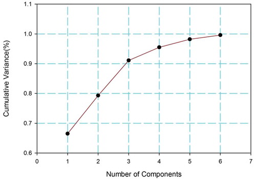
Table 1. Model scenario. See Table 2 for attributes

Properties	Description
Model	Data model
Period	1995–2016 (22 years)
Number of samples	8036 (1148 weeks)
Total number of attributes	6 + 1 (predicted label – ETo)
Attribute list	RHMX, RHMN, WS, TMAX, TMIN, SSH, ETo

Table 2. Statistical description of data model employed

Attribute	Description	Data type	Min	Max	Mean
RHMX (%)	Maximum relative humidity	Real	70	100	81.589
RHMN (%)	Minimum relative humidity	Real	33	100	59.267
WS (m s^−1)	Wind speed	Real	0.5	12.9	5.895
TMAX (°C)	Maximum temperature	Real	23	41.4	34.395
TMIN (°C)	Minimum temperature	Real	16	28.5	23.729
SSH (h)	Sunshine hours	Real	0	10.5	7.272
ETo (mm)	Reference evapotranspiration	Real	4.996	1.3472	3.890

Table 3. Attribute weights on selected principal components (PC)

Attribute	PC1	PC2	PC3
RHMX	−0.804	−0.132	−0.328
RHMN	−0.369	0.013	−0.919
WS	0.195	0.969	0.052
TMAX	0.256	0.194	0.094
TMIN	0.322	0.13	0.068
SSH	−0.1	−0.13	0.003

Figure 3. Attribution of weights in principal components

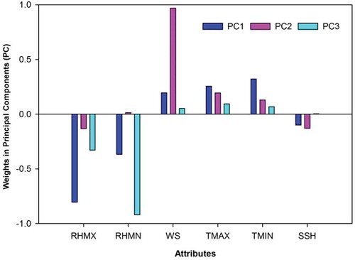
Table 4. Scenario of the reduced-features data model

Properties	Description
Number of samples	8036 (1148 weeks)
Total number of attributes	3 + 1 (predicted label – ETo)
Reduced attribute list	TMAX, TMIN, WS
Prediction attribute	ETo
Number of training samples	6429 samples (80% of actual samples)
Number of training samples	1607 samples (20% of actual samples)

Table 5. Parameter optimization of the radial basis function neural network (RBFNN) architecture. MSE: mean squared error. Best values are indicated in bold

Number of clusters	MSE for training	MSE for testing
10	0.15	0.10
20	0.8	0.06
30	0.11	0.08
40	0.17	0.11
50	0.20	0.15

Table 6. Variation of mean squared error (MSE) with the number of convolution layers (conv) and fully connected (full) layers of the convolutional neural network (CNN). Bold formatting indicates the optimum number of layers

Number of layers	MSE for training	MSE for testing
1 conv, 1 full	0.25	0.25
1 conv, 2 full	0.22	0.23
2 conv, 1 full	0.19	0.22
2 conv, 2 full	0.36	0.32

Table 7. Variation of the mean squared error (MSE) with the number of neurons in the fully connected layer of the convolutional neural network (CNN). Bold formatting indicates the optimum number of neurons

Number of neurons	MSE for training	MSE for testing
20	0.21	0.26
30	0.24	0.22
40	0.33	0.21
50	0.35	0.22
60	0.35	0.26

Table 8. Parameter values of the convolutional neural network (CNN) used in this study

Parameter	Value
Number of filters in convolutional layer	42
Kernel size	3
Dropout rate	0.1
Learning rate	0.001
Batch size	512
Learning model	Adam
Number of epochs	100

Table 9. Performance metrics for the artificial neural network (ANN) methods used in this study. DLNN: deep learning neural network; MAE: mean absolute error; RBFNN: radial basis function neural network; RMSE: root mean square error

Data model	Method	MAE		RMSE
Training	RBFNN	0.18	0.24
	DLNN	0.12	0.17
Testing	RBFNN	0.27	0.31
	DLNN	0.16	0.21

Table 10. Time taken to build the artificial neural network (ANN) methods. DLNN: deep learning neural network; RBFNN: radial basis function neural network

Data model	Method	Time taken (ms)
Training	RBFNN	1.05
	DLNN	3.43
Testing	RBFNN	0.04
	DLNN	2.9

Table 11. Comparison of the artificial neural network (ANN) methods by regression coefficient, R². DLNN: deep learning neural network; RBFNN: radial basis function neural network

Data model	Method	R^2
Training	RBFNN	0.952
	DLNN	0.991
Testing	RBFNN	0.862
	DLNN	0.979

Figure 4. Scatterplots of DLNN and RBFN models for (a) the training dataset and (b) the testing dataset

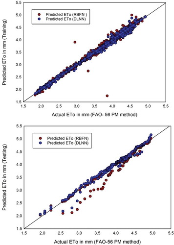
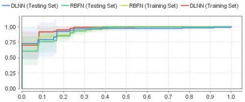
Figure 5. Receiver operating characteristic (ROC) curve of the DLNN and RBFN models (training and testing)