Infilling missing data of binary geophysical fields using scale invariant properties through an application to imperviousness in urban areas

Figures & data

Figure 1. Examples in one dimension (up) or two dimensions (bottom) of fields generated through the implementation of a β-model with various c

Figure 2. Illustration with a simple case of the successive steps of the conditional β-model. Ones are represented in black, zeros in white, and unknown/missing values in gold. (a) Start of the process: some data is missing and all the underlying increments of the process are unknown. (b) Filling the ones: all the increments needed to retrieve the ones of the original field are set to one. (c) Filling the zeros: a limited number of increments ensuring the zeros of the original field are retrieved are set to zero. (d) The remaining unknown increments are randomly drawn by using the probability distribution of Equation (5)(5) $Pr\left(\mu \epsilon ={\lambda }_1^c\right)={\lambda }_1^{-c}$(5) . More details (including the edge colour highlights can be found in the text

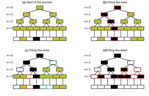
Figure 3. Outputs in one dimension of the conditional β-model for an initial field (top) simulated with c = 0.2. The content for each sub-figure is described through the title above it (more details can be found in the text). With regard to the “partial field” sub-figure, the yellow time steps correspond to the missing data (i.e. the time steps whose content has been artificially removed). With regard to the “Average over realizations” sub-figure, the colour scale goes from 0 (white) to 1 (black) through various levels of grey, and the gold line is simply a representation of the same information as a time series

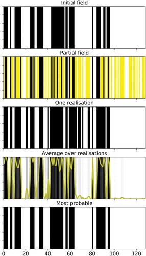
Figure 4. Computation of the fractal dimension (i.e. Equation (2)(2) $N_{\lambda ,A}\approx {\lambda }^{D_F}$(2) in log-log) of the initial field displayed in Fig. 3 (top row)

Figure 5. Outputs in two dimensions of the conditional β-model for an initial field simulated with c = 0.2

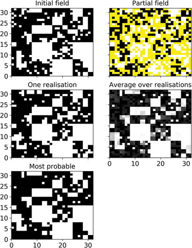
Figure 6. Percentage of hits on the missing data as a function of the proportion p of missing time steps inserted in the initial one-dimensional series for c = 0.1. Black lines indicate the average over realizations while red ones show the most probable fields. Solid lines show the 50% quantile over the 200 samples of initial fields while the dashed lines correspond to the 10 and 90% quantiles

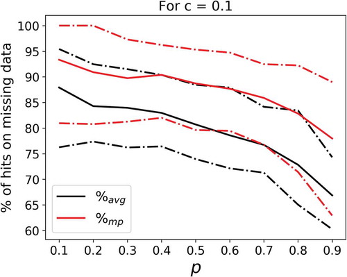
Figure 7. Percentage of hits on the missing data as a function of the proportion p of missing time steps inserted in the initial one-dimensional series for various values of c. Only the 50% quantile over a set of 200 samples of initial fields through the “most probable” approach are plotted (solid red line in Fig. 6)

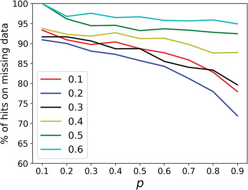
Figure 8. Evolution of c and ${\mathrm{\%}}_{mp}$ as a function of the number of iterations in the algorithm to run the conditional β-model when c is unknown. The initial field was generated with c = 0.2 and p = 0.7. The algorithm was started with c equal to 0 (black), 0.3 (blue) and 1 (green)

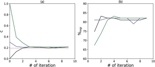
Figure 9. Temporal evolution of the rain rate corresponding to the 5 min time step studied rainfall series. Its length is of 2048 time steps, which corresponds to a duration of roughly 7.1 d. The series starts on 2019-06-02 00:00:00 (UTC)

Figure 10. Computation of the fractal dimension (i.e. Equation (2)(2) $N_{\lambda ,A}\approx {\lambda }^{D_F}$(2) in log-log) of the rainfall time series displayed in Fig. 9

Figure 11. Outputs in one dimension of the conditional β-model as in Fig. 3 with an “initial” field consisting of the rainfall time series displayed in Fig. 9

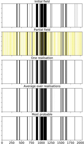
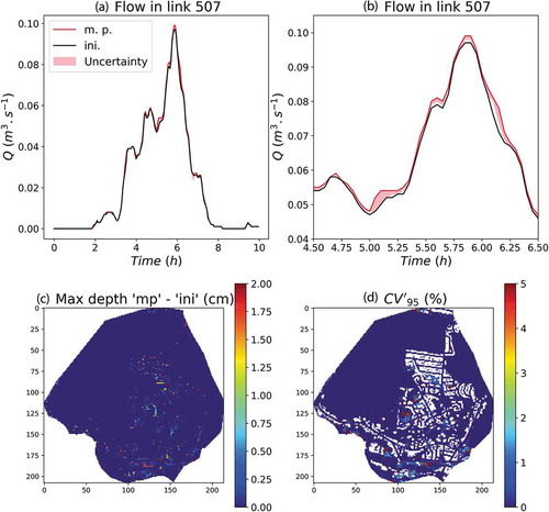
Figure 12. Representation of the Jouy-en-Josas catchment in Multi-Hydro with 2 m pixels. (a) “Initial” data, hence with missing data. (b) “Most probable” field, where missing data has been replaced by either grass or an impervious area using the developed conditional β-model

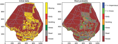
Figure 13. Same as in Fig. 12 size 10 m

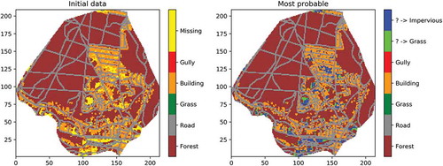
Figure 14. Computation of the fractal dimension (i.e. Equation (2)(2) $N_{\lambda ,A}\approx {\lambda }^{D_F}$(2) in log-log) of the geometrical set made of the impervious areas of the studied catchment with 2 m pixels (i.e. the field displayed in Fig. 12)

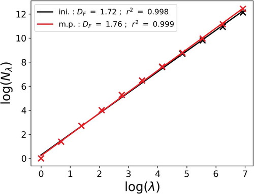
Figure 15. Outcome of the hydrodynamic simulations carried out with the Multi-Hydro model. “Initial” land-use data with the missing data taken as “grass” is used as input along with the 100 realizations of realistic ways of filling the 5.6% missing data, and the “most probable” field. (a) Simulated flows at link #507. Time is indicated since the beginning of the simulation. (b) Zoom of (a) near the peak flow. (c) Map of the difference in simulated maximum water depth between simulations carried out with the “most probable” field and the “initial” one. (d) Map of the $CV{ }_{95}^{\prime }$ coefficient for the maximum water depth