Daily streamflow prediction in ungauged basins: an analysis of common regionalization methods over the African continent

Figures & data

Table 1. Statistics of the catchment descriptors

Catchment descriptors used in regionalization	Minimum	Maximum	Median	Mean
Mean elevation (m)	32	2550	574	770
Drainage area (km^2)	303	3.65x10^6	6960	64,900
Average slope (%)	0.7	38	3.4	5.5
Land use – Forest (%)	0	98.2	0	4.12
Land cover – Grasslands (%)	0	100	0.32	9.94
Land cover – Savannas (%)	0	100	65.54	54.12
Mean annual precipitation, P (mm)	130	2118	1005	957
Aridity index (P/PET)	0.097	1.268	0.666	0.639
Other catchment properties not used in regionalization	Minimum	Maximum	Median	Mean
Mean annual PET (mm) *	745	1.92x10^3	1.61x10^3	1.49x10^3
Average streamflow, Q (m^3/s) *	0.021	3.98x10^4	16.83	261.3
Runoff ratio (Q/P) *	1.97x10^−4	0.746	0.092	0.129

* PET is used to compute the aridity index but is not used on its own for regionalization. The average streamflow and runoff ratio are for analysis only and not used for regionalization because, by definition, flow and runoff is not available at ungauged sites.

Figure 1. Land cover of Africa with the boundaries of the 314 catchments used in this study. MODIS land cover classes were combined into simpler classes (all types of forest are considered in the “Forest” class), and some minor and insignificant classes (urban, wetlands, snow/ice) were not added to the legend

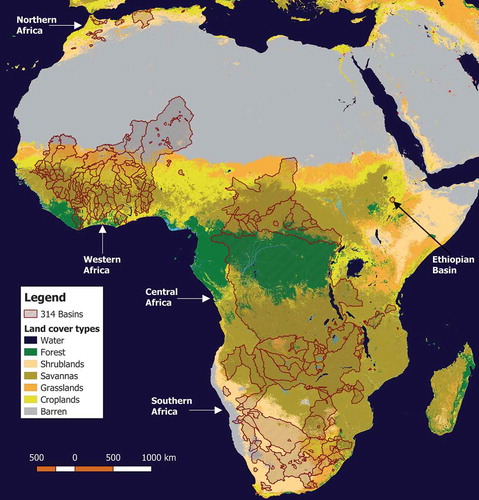
Figure 2. Average annual precipitation for each of the 314 African catchments used in this study. The large spatial variability of precipitation within and across regions can be noted

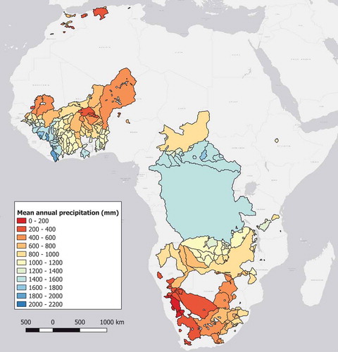
Figure 3. Calibration KGE for the 314 catchments. Three catchments have −0.25 < KGE < 0; 30 catchments have 0 < KGE < 0.4; 32 catchments have 0.4 < KGE < 0.6; 96 catchments have 0.6 < KGE < 0.8; and 156 catchments have KGE > 0.8

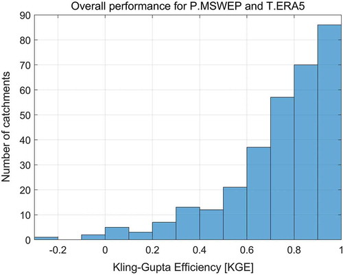
Figure 4. Spatial distribution of the calibration KGE values of the 314 catchments over Africa. Note that the larger catchments typically see better calibration KGE values than smaller catchments, except for the Niger River which is one of the worst in the dataset (KGE of −0.08)

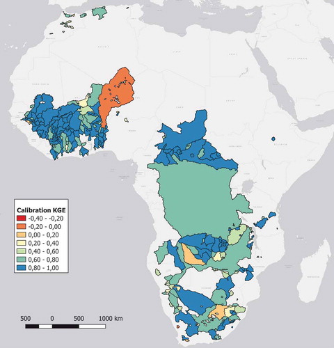
Table 2. Calibration KGE for different catchment size categories

Size lower bound (km^2)	Size upper bound (km^2)	Number of basins in group	Average calibration KGE score
-	1000	40	0.61
1000	5000	98	0.69
5000	10,000	42	0.77
10,000	100,000	89	0.82
100,000	-	45	0.77*
	Total	314	0.74

* Includes Niger River, with KGE = −0.08. Average becomes 0.79 when Niger River is excluded.

Figure 5. KGE of multiple donor averaging generated hydrographs using the IDW approach for SP (top panel) and PS (bottom panel). Note that improvements plateau at approximately four or five donors for both methods. The x-axis indicates the number of donors that were weighted (Wt1 = one donor, Wt2 = two donors, etc.). The MLR box plot indicates the performance of the MLR method over the study domain and is identical in both panels

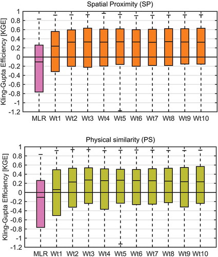
Figure 6. Spatial distribution of the three regionalization methods’ behaviour for the 314 catchments. Each dot’s color represents the ratio between the regionalized (Wt5) and the calibrated (Cal) KGE score for a given pseudo-catchment. The SP and PS regionalization KGE reflects that obtained by using the 5-donor weighted average

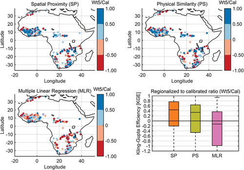
Figure 7. Catchments removed from the list of donors following the skill-based filtering. The three panels present the case with all donors (314 donors, left panel), with the KGE > 0.6 filter (250 donors, centre panel) and with the KGE > 0.8 filter (156 donors, right panel). Note that all North Africa and many Southern African catchments are removed with KGE > 0.8

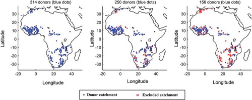
Figure 8. Spatial proximity (SP) regionalization KGE with skill-based filtering; row (a) regionalizing on all 314 pseudo-ungauged basins, row (b) regionalizing only on the subset of pseudo-ungauged basins that also pass through the filter (regionalizing only on well-calibrated pseudo-ungauged basins), and row (c) using all catchments as donors but regionalizing only on the “well-calibrated” catchments. The left column represents the base case (using all donors on all targets, and all three graphs are therefore identical), the centre column applies the first filter (KGE > 0.60) and the right column applies the second filter (KGE > 0.80). Titles indicate the number of donors and pseudo-ungauged targets used. Each panel has 5 box-plots: “Cal” is the calibration KGE for comparison purposes, “Near_1” is the regionalization KGE using the nearest single donor catchment, “Near_5” is the regionalization KGE using only the 5^th nearest donor catchment, “Wt5” is the weighted 5-donor KGE and “Wt5/Cal” represents the Wt5/Cal ratio to scale the results as a function of the maximum possible attainable skill (i.e. the calibration skill)

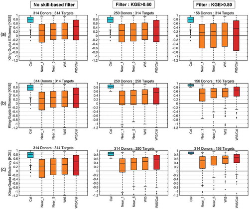
Figure 9. Same as Fig. 8 but for the physical similarity (PS) method

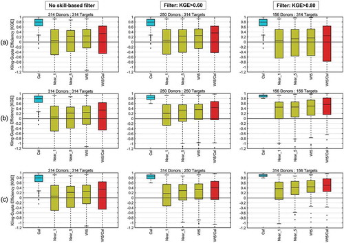
Figure 10. Same as Fig. 8 but for the multiple linear regression (MLR) regionalization method. Each panel presents the calibration KGE, the MLR KGE and the ratio of MLR/Calibration

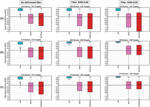
Table 3. Correlation coefficients between regionalization KGE and the catchment descriptors used in regionalization

	Drainage area	Mean slope	Elevation	Forests	Grass-	Savannas	Ann. Precip.	Aridity
					lands			index
SP_5 Wt	0.01	0.04	−0.08	0.04	0.02	0.07	0.11	0.09
PS_5 Wt	0.03	0.07	−0.08	0.05	−0.01	0.09	0.18	0.18
MLR	0.02	0.02	0.08	−0.13	0.03	0.08	−0.17	−0.15

Table 4. Average distance (in kilometers) between the ungauged catchment and its nearest donor based on the filtering level for both the SP and PS methods

Filter level	Number of donors left	SP (centroid distance, km)	PS (centroid distance, km)	PS (similarity index, unitless)
No filter	314 donors	140.65	339.11	0.364
KGE > 0.60	250 donors	167.63	371.2	0.398
KGE > 0.80	156 donors	370.55	572.11	0.504