Figures & data
Figure 1. Map presenting the study area, the Euro-CORDEX grid, and the raingauges and thermometers used to assess model errors in reproducing climate statistics for the control period (1971–2000). Many of the temperature records are available at the same location as the raingauges.
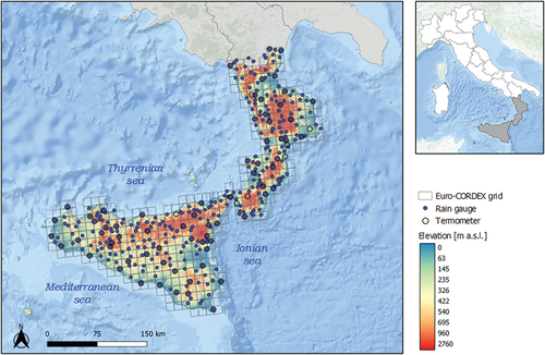
Table 1. Five most accurate Euro-CORDEX climate models for the study area.
Table 2. Predetermined combinations of error metric exponents for weight calculations.
Figure 2. Sketch illustrating the traditional (static) approach versus the proposed dynamic approach for assessing the impacts of climate change on droughts based on standardized indices. The sketch refers to 1971–2000 as the control period and 2041–2070 as future periods, but it is valid for other periods also. It should be noted that reference periods belong entirely to historical or to future scenario periods, as mixed historical–future scenario periods are non-stationary by definition and climate normals cannot be defined.
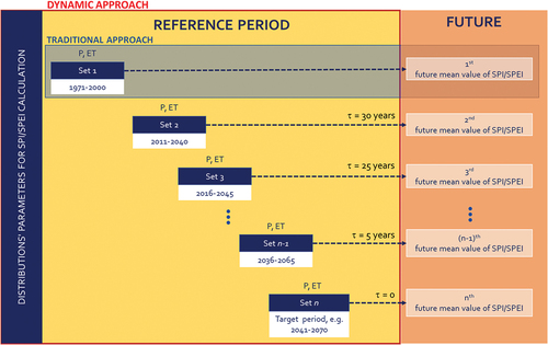
Table 3. Errors in climate reproduction by single climate models and their combinations.
Table 4. Spatially averaged changes (∆) and relative climate model uncertainty (weighted standard deviation) of mean annual precipitation, temperature and reference evapotranspiration for Sicily, Calabria and the entire study area.
Figure 3. Monthly variations of precipitation and reference evapotranspiration (OWEA and single CMs). Temperature variations are qualitatively similar to those of evapotranspiration, and thus are not shown.
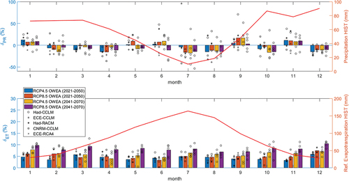
Figure 4. Projected changes in mean annual precipitation.
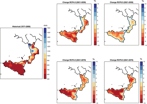
Figure 5. Projected changes in mean annual temperature.
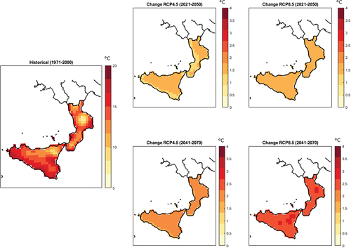
Figure 6. Projected changes in mean annual reference evapotranspiration.
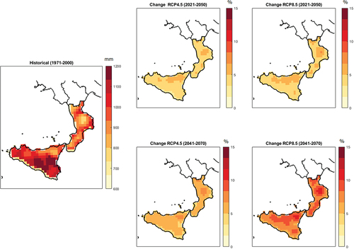
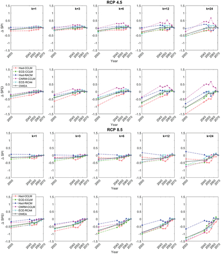
Figure 7. Projected changes in SPI at increasing time aggregation scales for different scenarios and future periods.
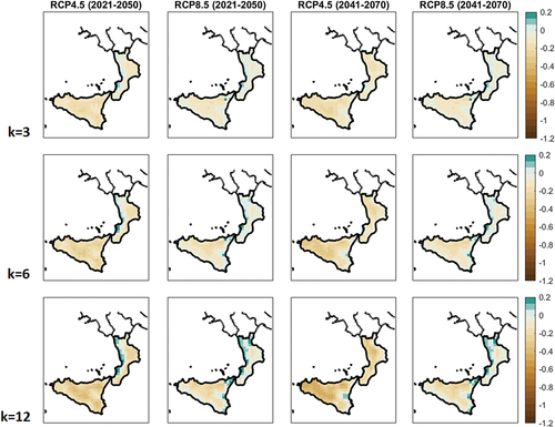
Figure 8. Projected changes in SPEI at increasing time aggregation scales for different scenarios and future periods.
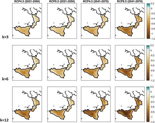
Table 5. Spatially averaged changes (∆) for the standardized precipitation index in Sicily, Calabria and the entire study area.
Table 6. Spatially averaged changes for the standardized precipitation and evapotranspiration index in Sicily, Calabria and the entire study area.
Figure 9. Plots showing the change in the average values of SPI and SPEI on moving time windows (x-axis represents the end year of the calibration period) and different time aggregations k (in months) for the whole investigated area (Calabria and Sicily).