Automatic water-level class estimation from repeated crowd-based photos of streams

Figures & data

Figure 1. Photographs illustrating the principle of the virtual staff gauge approach used in the CrowdWater project. The first observer at a location (i.e. spot) takes a photo that shows the water surface and a reference object (in this case a pile of rocks) and inserts the virtual staff gauge (a sticker) in the photo, in such a way that class 0 (blue line) is on the water surface (a). The same observer or other observers can take photos of the spot at a later time and determine the new water-level class by looking at the position of the water surface relative to the reference objects (b–g) and the virtual staff gauge on the initial photo (a). Photos and data from https://www.spotteron.com/crowdwater/spots/23 445.

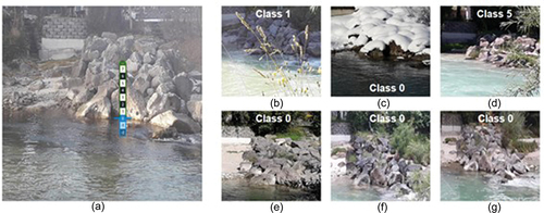
Figure 2. Schematic representation of the dataset construction. The dataset consisted of pairs of photos: the initial photo with virtual staff gauge and a photo at the same spot taken at a later time (see Fig. 1). The citizen scientist who submitted the second photo also submitted a value for the water-level class. The photo pairs were then evaluated in the CrowdWater game, where multiple citizen scientists cast their vote on the water-level class for the second photo. The median of these votes was used as the label for the classification task, while the classes with the highest and second-highest number of votes (see Equations 1(1) $\begin{array}{rl}& C_{\mathrm{h}\mathrm{i}\mathrm{g}\mathrm{h}-\mathrm{r}\mathrm{e}\mathrm{s}\mathrm{o}\mathrm{l}\mathrm{u}\mathrm{t}\mathrm{i}\mathrm{o}\mathrm{n}}=C_{\mathrm{m}\mathrm{a}\mathrm{x}}-\frac{N_{\mathrm{s}\mathrm{e}\mathrm{c}\mathrm{o}\mathrm{n}\mathrm{d}-\mathrm{m}\mathrm{a}\mathrm{x}}}{N_{\mathrm{m}\mathrm{a}\mathrm{x}}+N_{\mathrm{s}\mathrm{e}\mathrm{c}\mathrm{o}\mathrm{n}\mathrm{d}-\mathrm{m}\mathrm{a}\mathrm{x}}}\\ & \mathrm{i}\mathrm{f}{C}_{\mathrm{m}\mathrm{a}\mathrm{x}}\ge C_{\mathrm{s}\mathrm{e}\mathrm{c}\mathrm{o}\mathrm{n}\mathrm{d}-\mathrm{m}\mathrm{a}\mathrm{x}}\end{array}$(1) and 2(2) $\begin{array}{rl}& C_{\mathrm{h}\mathrm{i}\mathrm{g}\mathrm{h}-\mathrm{r}\mathrm{e}\mathrm{s}\mathrm{o}\mathrm{l}\mathrm{u}\mathrm{t}\mathrm{i}\mathrm{o}\mathrm{n}}=C_{\mathrm{m}\mathrm{a}\mathrm{x}}+\frac{N_{\mathrm{s}\mathrm{e}\mathrm{c}\mathrm{o}\mathrm{n}\mathrm{d}-\mathrm{m}\mathrm{a}\mathrm{x}}}{N_{\mathrm{m}\mathrm{a}\mathrm{x}}+N_{\mathrm{s}\mathrm{e}\mathrm{c}\mathrm{o}\mathrm{n}\mathrm{d}-\mathrm{m}\mathrm{a}\mathrm{x}}}\\ & \mathrm{i}\mathrm{f}{C}_{\mathrm{m}\mathrm{a}\mathrm{x}}<C_{\mathrm{s}\mathrm{e}\mathrm{c}\mathrm{o}\mathrm{n}\mathrm{d}-\mathrm{m}\mathrm{a}\mathrm{x}}\end{array}$(2) ) were used as the label for the regression task. For both tasks, the data for the very high and very low water-level classes were merged in the reclassification process to reduce the number of classes for which there were very few observations. The dataset was divided into a training set and a test (or validation) set, with 80% and 20% of all photos for each spot and class, respectively.

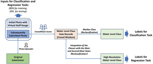
Figure 3. (a) Number of photos for the different water-level classes after reclassification to nine classes, and (b) the cumulative probability curve for the higher resolution water-level class data (see Equations 1(1) $\begin{array}{rl}& C_{\mathrm{h}\mathrm{i}\mathrm{g}\mathrm{h}-\mathrm{r}\mathrm{e}\mathrm{s}\mathrm{o}\mathrm{l}\mathrm{u}\mathrm{t}\mathrm{i}\mathrm{o}\mathrm{n}}=C_{\mathrm{m}\mathrm{a}\mathrm{x}}-\frac{N_{\mathrm{s}\mathrm{e}\mathrm{c}\mathrm{o}\mathrm{n}\mathrm{d}-\mathrm{m}\mathrm{a}\mathrm{x}}}{N_{\mathrm{m}\mathrm{a}\mathrm{x}}+N_{\mathrm{s}\mathrm{e}\mathrm{c}\mathrm{o}\mathrm{n}\mathrm{d}-\mathrm{m}\mathrm{a}\mathrm{x}}}\\ & \mathrm{i}\mathrm{f}{C}_{\mathrm{m}\mathrm{a}\mathrm{x}}\ge C_{\mathrm{s}\mathrm{e}\mathrm{c}\mathrm{o}\mathrm{n}\mathrm{d}-\mathrm{m}\mathrm{a}\mathrm{x}}\end{array}$(1) and 2(2) $\begin{array}{rl}& C_{\mathrm{h}\mathrm{i}\mathrm{g}\mathrm{h}-\mathrm{r}\mathrm{e}\mathrm{s}\mathrm{o}\mathrm{l}\mathrm{u}\mathrm{t}\mathrm{i}\mathrm{o}\mathrm{n}}=C_{\mathrm{m}\mathrm{a}\mathrm{x}}+\frac{N_{\mathrm{s}\mathrm{e}\mathrm{c}\mathrm{o}\mathrm{n}\mathrm{d}-\mathrm{m}\mathrm{a}\mathrm{x}}}{N_{\mathrm{m}\mathrm{a}\mathrm{x}}+N_{\mathrm{s}\mathrm{e}\mathrm{c}\mathrm{o}\mathrm{n}\mathrm{d}-\mathrm{m}\mathrm{a}\mathrm{x}}}\\ & \mathrm{i}\mathrm{f}{C}_{\mathrm{m}\mathrm{a}\mathrm{x}}<C_{\mathrm{s}\mathrm{e}\mathrm{c}\mathrm{o}\mathrm{n}\mathrm{d}-\mathrm{m}\mathrm{a}\mathrm{x}}\end{array}$(2) ). These frequency curves show the data for all 385 spots combined.

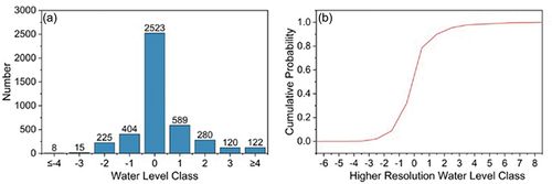
Figure 4. Schematic illustration of the steps used in model training and evaluation in this study. In the training stage, the model used photo pairs from the training dataset (80% of all photo pairs) as input, predicted the water-level class, calculated the loss function based on the true values, and updated the model parameters using different training strategies (semi-trained or fully-trained). In the evaluation stage, the trained model predicted the water-level class for the photo pairs from the test dataset (20% of all photo pairs), and the results were compared to the true water-level class (i.e. water-level class from the game) to calculate the evaluation metrics. These metrics were also calculated for the water-level class provided by the citizen scientist who uploaded the photo.

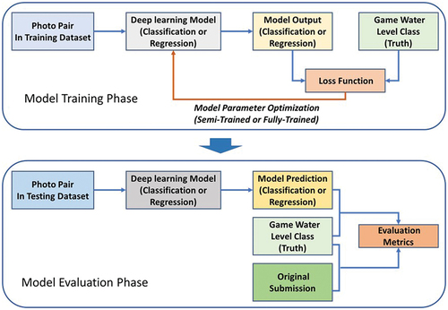
Figure 5. Set-up of the model used in this study. The model is composed of two parts: the feature extraction module and classifier module. The initial photo with the virtual staff gauge and the photo taken at the same spot at a later time go through the feature extraction module separately. The extracted features are subsequently concatenated and processed in the second module to accomplish the classification or regression task. The feature extraction module follows the VGG 19 model and is constructed by stacking multiple convolution layers and max pooling layers. The classifier module mainly depends on a series of fully-connected layers. The ReLU function was used after each convolution layer. The height, width and channel number of the input images and vectors in each step are indicated in the figure.

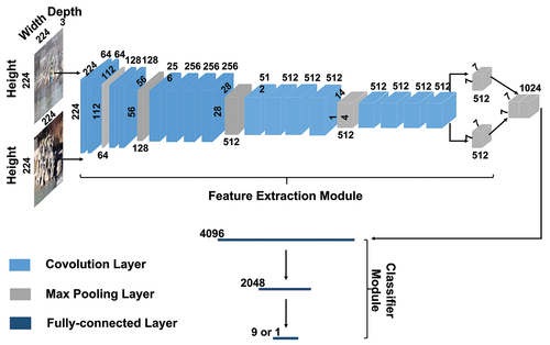
Figure 6. Schematic representation of the convolution and max-pooling operation in the CNN model.

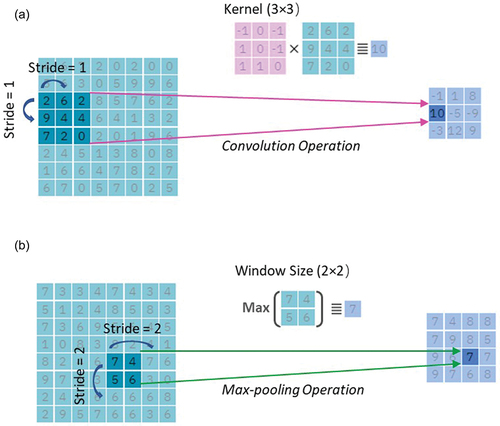
Figure 7. Box plots of (a) the root mean square error R and (b) the Spearman rank correlation coefficient r_s for of the fully-trained and semi-trained models for the classification task and for the water-level class estimated by the citizen scientist who submitted the photo. R was calculated for all 385 spots, while r_s could only be evaluated for the 112 spots for which the water-level class varied over at least two classes. The median vote for a photo in the CrowdWater game was assumed to be the truth. The upper and lower boundary of the box represent the upper (0.75) and lower (0.25) quartiles, the solid line is the median, the whiskers extend to 1.5 times the interquartile range, and the dots are outliers.

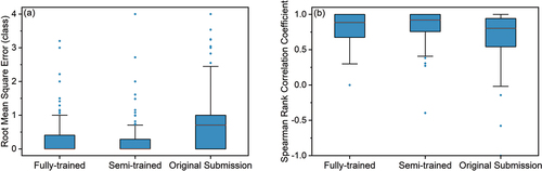
Table 1. The accuracy (A [-]) and root mean square error (R [classes]) for the testing dataset for images with different water-level classes.

Water-level class	Number of images n	Fully-trained model		Semi-trained model		Original submission
		A	R	A	R	A	R
−4	2	1.00	0.00	1.00	0.00	1.00	0.00
−3	4	1.00	0.00	0.25	0.87	0.25	0.87
−2	46	0.76	0.55	0.80	0.51	0.50	1.22
−1	82	0.70	0.76	0.65	0.65	0.45	1.14
0	506	0.76	0.59	0.79	0.55	0.59	0.99
1	119	0.54	0.86	0.52	0.85	0.60	0.76
2	57	0.56	0.89	0.51	0.97	0.44	0.96
3	25	0.44	1.11	0.24	1.36	0.52	0.69
4	25	0.32	1.64	0.68	1.56	0.88	0.35

Figure 8. Relation between the Spearman rank correlation coefficient r_s for the water-level class identified by the citizen scientists who submitted the photo (x-axis) and the semi-trained model (y-axis) for the 56 spots for which observations were available for at least two different water-level classes after excluding the class 0 observations. The median of the vote for an image in the CrowdWater game was used as the truth. The shapes of the spots in (a) indicate the variance, and in (b) they show the range of water-level class observations. The result for the one spot for which the r_s is negative is not shown.

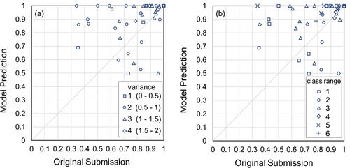
Figure 9. The water-level class based on the median vote from the game (i.e. ground truth; blue line) for all the analysed photos, and the corresponding semi-trained model predictions (red dot) and original submissions (green triangle) where they do not match the ground truth for two example spots (Location 1 (a) and 2 (b)). For visualization, only the results for the wrongly classified photos are shown; those that were predicted correctly by the model or submitted correctly by the citizen scientists are not shown (and would plot on the blue line). The photo numbers are in chronological order, but the time interval between adjacent photos differs.

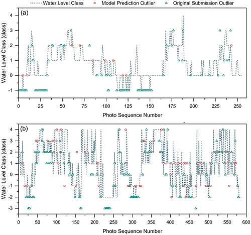
Figure 10. Example photos for two spots for which the model performance was not satisfactory: photos taken (a) from a moving train resulting in a negative Spearman rank correlation coefficient r_s for both the model and the original observation (photos from: https://www.spotteron.com/crowdwater/spots/40237), and (b) for a spot where the Spearman rank correlation is lower for the model than for the original submission because the sight distance and visual angle differ considerably from one photo to another (photos from: https://www.spotteron.com/crowdwater/spots/22036).

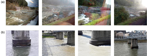
Figure 11. Box plots of (a) the root mean square error R and (b) the Spearman rank correlation coefficient r_s of the water-level class time series for the classification and regression models (semi-trained). R was calculated for all 385 spots, and r_s only for the 112 spots for which the water-level class varied over at least two classes. For the classification task, the photos were compared with the median vote from the CrowdWater game. For the regression task, the classes with the most and the second most votes in the game were used to derive higher resolution class data for the photos (see Fig. 2 for a schematic representation). Note that the result for the one outlier for the classification model with a root mean square error of 4.8 classes is not shown.

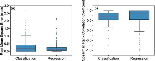
Figure 12. The water-level class data (Equations 1(1) $\begin{array}{rl}& C_{\mathrm{h}\mathrm{i}\mathrm{g}\mathrm{h}-\mathrm{r}\mathrm{e}\mathrm{s}\mathrm{o}\mathrm{l}\mathrm{u}\mathrm{t}\mathrm{i}\mathrm{o}\mathrm{n}}=C_{\mathrm{m}\mathrm{a}\mathrm{x}}-\frac{N_{\mathrm{s}\mathrm{e}\mathrm{c}\mathrm{o}\mathrm{n}\mathrm{d}-\mathrm{m}\mathrm{a}\mathrm{x}}}{N_{\mathrm{m}\mathrm{a}\mathrm{x}}+N_{\mathrm{s}\mathrm{e}\mathrm{c}\mathrm{o}\mathrm{n}\mathrm{d}-\mathrm{m}\mathrm{a}\mathrm{x}}}\\ & \mathrm{i}\mathrm{f}{C}_{\mathrm{m}\mathrm{a}\mathrm{x}}\ge C_{\mathrm{s}\mathrm{e}\mathrm{c}\mathrm{o}\mathrm{n}\mathrm{d}-\mathrm{m}\mathrm{a}\mathrm{x}}\end{array}$(1) and 2(2) $\begin{array}{rl}& C_{\mathrm{h}\mathrm{i}\mathrm{g}\mathrm{h}-\mathrm{r}\mathrm{e}\mathrm{s}\mathrm{o}\mathrm{l}\mathrm{u}\mathrm{t}\mathrm{i}\mathrm{o}\mathrm{n}}=C_{\mathrm{m}\mathrm{a}\mathrm{x}}+\frac{N_{\mathrm{s}\mathrm{e}\mathrm{c}\mathrm{o}\mathrm{n}\mathrm{d}-\mathrm{m}\mathrm{a}\mathrm{x}}}{N_{\mathrm{m}\mathrm{a}\mathrm{x}}+N_{\mathrm{s}\mathrm{e}\mathrm{c}\mathrm{o}\mathrm{n}\mathrm{d}-\mathrm{m}\mathrm{a}\mathrm{x}}}\\ & \mathrm{i}\mathrm{f}{C}_{\mathrm{m}\mathrm{a}\mathrm{x}}<C_{\mathrm{s}\mathrm{e}\mathrm{c}\mathrm{o}\mathrm{n}\mathrm{d}-\mathrm{m}\mathrm{a}\mathrm{x}}\end{array}$(2) ) and regression model estimates for two spots (Location 1 and 2). The photo numbers are in chronological order, but the time interval between adjacent photos differs.

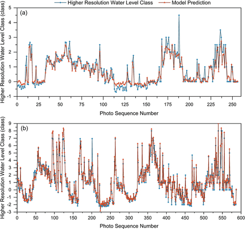
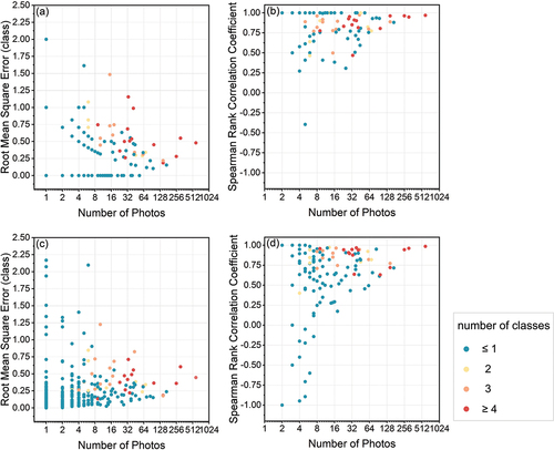
Figure 13. Influence of the number of training photos on model performance in terms of root mean square error R (a and c) and Spearman rank correlation coefficient r_s (b and d) for the classification task (a, b) and regression task (c, d). Each dot represents one spot and is coloured by the number of classes over which the water level varied in the photos for that spot.

Data availability statement

The data used in this study were collected by the citizen scientists of the CrowdWater project and can be downloaded from https://crowdwater.ch/en/data/.