The uncertainty associated with the use of copulas in multivariate analysis

Figures & data

Table 1. Parameter ranges and the relation between $\mathit{\theta }$ and Kendall’s $\mathit{\tau }$, where $D_1\left(\mathit{\theta }\right)$ is the first Debye function (Abramowitz and Stegun 1970).

Copula family	Parameter range	Relation between $\mathit{\theta }$ and Kendall’s $\mathit{\tau }$
Frank	$-\mathrm{\infty }<\mathit{\theta }<\mathrm{\infty }$, $\mathit{\theta }\ne 0$	$\mathit{\tau }=1-\frac{4\left(1-D_1\left(\mathit{\theta }\right)\right)}{\mathit{\theta }}$
Gumbel	$1\le \mathit{\theta }<\mathrm{\infty }$	$\mathit{\tau }=1-\frac{1}{\theta }$
Clayton	$-1\le \mathit{\theta }<\mathrm{\infty }$	$\mathit{\tau }=\frac{\theta }{\mathit{\theta }+2}$

Table 2. Copula parameter $\mathit{\theta }$ for given Kendall’s $\mathit{\tau }$.

Copula τ	$0.1$	$0.3$	$0.5$	$0.7$	$0.9$
Frank	$0.91$	$2.92$	$5.74$	$11.41$	$38.28$
Gumbel	$1.11$	$1.43$	$2.00$	$3.33$	$10.00$
Clayton	$0.22$	$0.86$	$2.00$	$4.67$	$18.00$

Figure 1. Scatter plots of a sample from a copula with τ =  0.1, 0.5, 0.9 and n =  100.

Figure 2. Example of confidence curves for τ for one of the synthetic samples for each copula with ${\tau }_{\mathrm{true}}$ = 0.1, 0.5, 0.9 and n = 100.

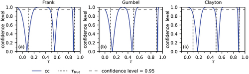
Figure 3. Box plots of $\hat{\tau }-{\mathit{\tau }}_{\mathrm{true}}$ for different copulas and different sample sizes.

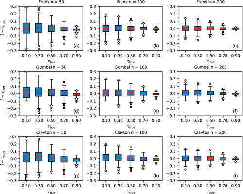
Figure 4. Box plots of $\left(\widehat{\theta }-{\theta }_{\text{true}}\right)$ for different copulas and different sample sizes.

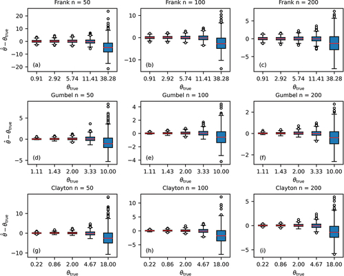
Table 3. Actual coverage probability (%) of a confidence interval with a nominal coverage probability of 95%.

Copula	τ n	$0.1$	$0.3$	$0.5$	$0.7$	$0.9$
Frank	$50$	$94.2$	$92.6$	$93.1$	$91.5$	$73.0$
	$100$	$95.0$	$93.2$	$92.6$	$92.0$	$84.6$
	$200$	$94.4$	$94.6$	$93.3$	$93.6$	$86.5$
Gumbel	$50$	$94.3$	$90.6$	$87.2$	$84.1$	$72.1$
	$100$	$94.0$	$90.2$	$87.4$	$85.5$	$74.6$
	$200$	$94.7$	$89.8$	$88.0$	$84.6$	$78.1$
Clayton	$50$	$92.0$	$86.5$	$85.1$	$78.5$	$62.3$
	$100$	$92.1$	$86.2$	$83.7$	$81.5$	$63.4$
	$200$	$93.1$	$88.1$	$82.6$	$79.4$	$64.1$

Figure 5. Actual coverage probability versus the nominal one for $\mathit{\tau }$ in copulas.

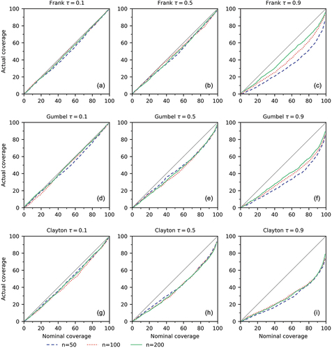
Figure 6. Box plots of the width of confidence intervals for a 95% confidence level.

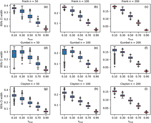
Figure 7. Box plots of the difference between the true value and the estimate of τ in the synthetic experiments with n = 200.

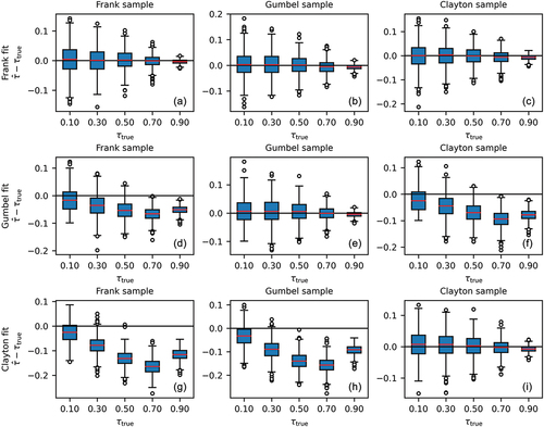
Figure 8. Station locations.

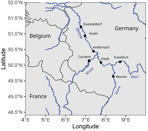
Table 4. Dependence parameters between time series and width of the 95% confidence intervals for the estimate of dependence parameter.

Time series pair	Frank		Clayton		Gumbel ${180}^{\circ }$		Galambos ${180}^{\circ }$		Huesler-Reiss ${180}^{\circ }$
	$\mathit{\theta }$	Width	$\mathit{\theta }$	Width	$\mathit{\theta }$	Width	$\mathit{\theta }$	Width	$\mathit{\theta }$	Width
Andernach and Koeln	59.0	21.7	20.3	7.8	14.7	5.1	14.0	5.1	16.4	5.0
Cochem and Kaub	8.0	3.8	2.3	1.3	2.5	0.9	1.8	0.9	2.2	0.8
Cochem and Worms	5.4	3.2	1.5	1.0	1.9	0.7	1.2	0.6	1.7	0.7
Worms and Frankfurt	4.6	3.8	1.2	1.1	1.7	0.7	1.0	0.7	1.5	0.8

Table 5. Kendall’s $\mathit{\tau }$ values between time series and width of the 95% confidence intervals.

Time series pair	Frank		Clayton		Gumbel ${180}^{\circ }$		Galambos ${180}^{\circ }$		Huesler-Reiss ${180}^{\circ }$
	$\mathit{\tau }$	Width	$\mathit{\tau }$	Width	$\mathit{\tau }$	Width	$\mathit{\tau }$	Width	$\mathit{\tau }$	Width
Andernach and Koeln	0.93	0.02	0.91	0.03	0.93	0.02	0.93	0.02	0.93	0.02
Cochem and Kaub	0.60	0.14	0.53	0.14	0.60	0.14	0.60	0.14	0.58	0.13
Cochem and Worms	0.48	0.19	0.43	0.16	0.48	0.18	0.48	0.18	0.47	0.16
Worms and Frankfurt	0.43	0.26	0.37	0.22	0.42	0.25	0.42	0.24	0.42	0.23

Figure 9. Confidence curves and scatter plots for pairs of stations. Discharge at the downstream station is indicated by the colour of the dots in the scatter plots.

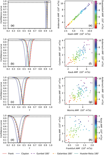
Figure 10. The pdfs for copulas for the station pair Cochem and Kaub.

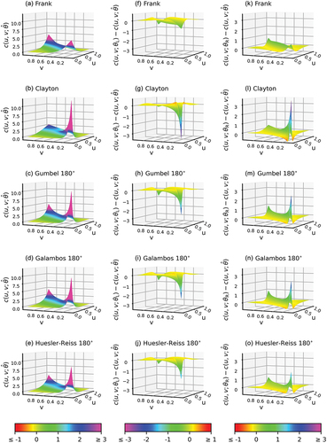
Figure 11. Location of the karst area. Both figures combine Google Map data ©2015 with material from Natural Earth.

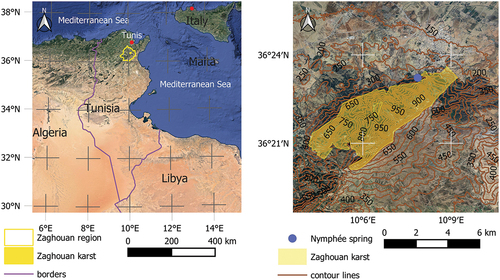
Figure 12. The hydrograph (curve) for Nymphée spring from 1924 to 1926. The figure also contains a monthly hyetograph (bars).

Figure 13. Daily rainfall, runoff, and shifted runoff.

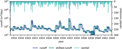
Figure 14. Kendall’s τ for different lags and confidence curves for the selected lag (CI = confidence interval).

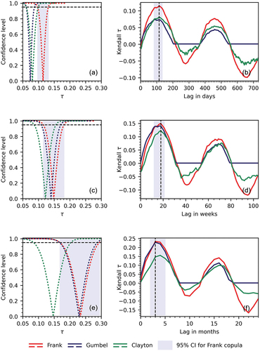
Table 6. Table of lags and confidence intervals.

Copula	Time step	$\hat{\tau }\left(\hat{m}\right)$	$\hat{m}$	90% interval	95% interval
Frank	Day	0.114	115	[86.0, 131.0]	[83.0, 133.0]
	Week	0.149	18	[13.0, 20.0]	[12.0, 21.0]
	Month	0.233	3	[3.0, 5.0]	[2.0, 5.0]
Clayton	Day	0.081	116	[85.0, 136.0]	[82.0, 141.0]
	Week	0.122	18	[13.0, 21.0]	[12.0, 22.0]
	Month	0.156	4	[3.0, 5.0]	[3.0, 6.0]
Gumbel	Day	0.074	87	[78.0, 125.0]	[75.0, 128.0]
	Week	0.140	17	[11.0, 19.0]	[11.0, 20.0]
	Month	0.229	3	[2.0, 4.0]	[2.0, 5.0]

Abramowitz, M. and Stegun, I.A., 1970. Handbook of mathematical functions. New York: Dover Publications Inc.

 Google Scholar