What interrupted monomictic mixing in Lake Biwa? Heat budget analysis using a circulation model

Figures & data

Figure 1. (a) Map of the area around Lake Biwa showing the watersheds and river paths. The blue shaded area indicates the watershed flowing into Lake Biwa in the Yodo River Basin (black shaded area) flowing into Osaka Bay (colour scale indicates depth in metres). The red square denotes the study area. (b) Topography and bathymetry of the area around Lake Biwa. The black square (17B) indicates the regular monitoring site (Imazu-oki-chuo) of the Lake Biwa Environmental Research Institute (LBERI). The black dot (M) indicates the Adogawa Offshore Comprehensive Automatic Observation Station of the Japan Water Agency (JWA).

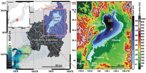
Table 1. Thickness and centre depth of layer at each level used in the model.

Layer #	Thickness (m)	Centre depth of layer (m)
1	3	1.5
2	2	4.0
3	2	6.0
4	2	8.0
5	2	10.0
6	2	12.0
7	2	14.0
8	2	16.0
9	2	18.0
10	2	20.0
11	3	22.5
12	3	25.5
13	3	28.5
14	4	32.0
15	4	36.0
16	4	40.0
17	4	44.0
18	4	48.0
19	4	52.0
20	4	56.0
21	4	60.0
22	4	64.0
23	4	68.0
24	4	72.0
25	5	76.5
26	5	81.5
27	5	86.5
28	5	91.5
29	5	96.5
30	5	101.5

Table 2. Sensitivity experiment for 12 cases in 2017/2018 and 2018/2019 with different perturbed values for the air temperature and wind speed with respect to sensible and latent heat fluxes.

Year	Property	Experimental case names
2017/2018	Air temperature
	Increases 1°C	Ta + 1°C
	Increases 2°C	Ta + 2°C
	Increases 3°C	Ta + 3°C
	Wind speed
	Decreases 10%	W – 10%
	Decreases 20%	W – 20%
	Decreases 30%	W – 30%
2018/2019	Air temperature
	Increases 1°C	Ta + 1°C
	Increases 2°C	Ta + 2°C
	Increases 3°C	Ta + 3°C
	Wind speed
	Increases 10%	W + 10%
	Increases 20%	W + 20%
	Increases 30%	W + 30%

Figure 2. Scatter plot showing the simulated and observed water temperatures at 17B, the fixed station (Fig. 1), during the cooling period in 2017/2018 and 2018/2019.

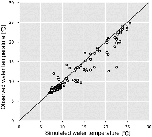
Figure 3. Hovmöller diagrams of the hourly vertical profiles of the simulated water temperatures (colour shades) during the cooling period from September to March in (a) 2017/2018 and (b) 2018/2019, and observed water temperatures (17B in Fig. 1) denoted by the coloured dots. White dots indicate the daily mean mixed layer depth (bottom of the mixed layer). Black column-like contours around mid-October in 2017 indicate the dense isotherms.

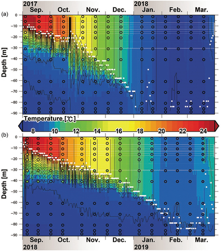
Figure 4. Maps of the monthly-mean simulated water temperature (colours) and velocity fields (vectors) in the surface layer at 4 m depth in (a) September 2017 and (b) September 2018, and the occurrence in days of simulated full overturn during the cooling period from September to the following March in (c) 2017/2018 and (d) 2018/2019.

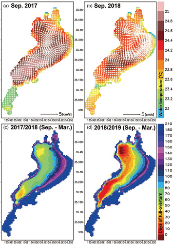
Figure 5. Heat budget and overturn analyses of Lake Biwa during the cooling periods in 2017/2018 (left panels) and 2018/2019 (right panels). Temporal variations in the 25 h running mean (upper panels) of the spatial occupancy of the overturn; total percentage areas of the simulated full overturn (A_FO) per entire lake area (670 km²) and the volume of the mixed layer (V_ML) per entire lake volume (27.5 km²). Middle panels: the surface heat flux areas are averaged over the whole lake; incoming solar radiation (S); net longwave radiation (L); sensible heat flux (H); latent heat flux (IE). Lower panels: the heat flux and heat storage of the lake; Bowen ratio (Br), net surface heat flux (QN), and heat storage (HS) corresponding to the mixing index (LaMIX) scaled by the vertical axis located between the panels. Lateral red lines indicate HS = 1000 in petajoules (PJ). White lines indicate LaMIX = 1 each year, indicating the monomictic mixing regime in the lake.

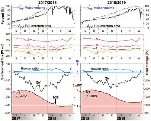
Figure 6. Time series of the cumulative surface heat flux, incoming solar radiation (S), net longwave radiation (L), sensible heat flux (H), and latent heat flux (IE) during the cooling period (September–March) in 2017/2018 (dotted lines) and 2018/2019 (solid lines).

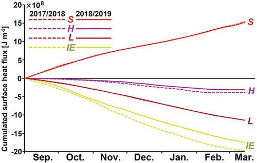
Figure 7. Time series of the 25 h running mean of (a) air temperature (T_a), surface water temperature (T_S), and their differences (∆T = T_a − T_s) to evaluate the contribution of temperature to H in Equation (4)(4) $H=c_p{\rho }_a{C}_{H}W\left(T_a-T_s\right)$(4) ; and (b) specific humidity (q_a), saturated specific humidity (q_S), and their difference (∆q = q_a − q_s) to evaluate the contribution of humidity to IE in Equation (5)(5) $IE=l{\rho }_a{C}_{E}W\left(q_a-q_s\right)$(5) during the cooling period (September–March) in 2017/2018 (dotted lines) and 2018/2019 (solid lines). All properties used for the time series were area averaged across the whole lake.

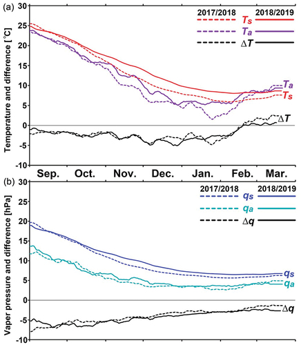
Figure 8. Time series of the 25 h running mean for wind speed (W) during the cooling period (September–March) in 2017/2018 (dotted lines) and 2018/2019 (solid lines); the differences (∆W) between W in 2017/2018 minus W in 2018/2019 were used to evaluate the differences in the magnitudes of H and IE. All properties used for the time series were area averaged across the whole lake.

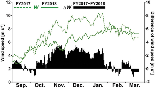
Table 3. Time-averaged values of the meteorological factors during the cooling period from September to the following March in 2017/2018 and 2018/2019, and the differences between years.

		2017/2018	2018/2019	Difference(2017–2018)
Temperature (°C)
Air temp.	Ta	10.6	11.8	−1.2
Water temp.	Ts	12.5	14.0	−1.5
Difference	Ta – Ts	−1.9	−2.2	0.3
Specific humidity
Actual	qa	5.5	5.9	−0.4
Saturated	qs	9.5	10.2	−0.7
Difference	qa – qs	−4.0	−4.4	0.3
Wind speed (m s^−1)
	W	7.5	6.2	1.3

Figure 9. Maps of the days of full-overturn occurrence (D_FO) in each case of the sensitivity experience (Table 2) during the cooling period from September to the following March in 2017/2018 and 2018/2019.

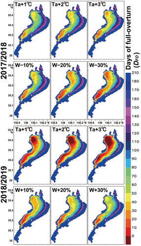
Figure A1. Scatter plots showing (a) predicted (GPV-MSM) and in situ air temperatures observed at the fixed meteorological station (M) (Fig. 1); and (b) predicted and in situ dew-point temperatures during the cooling periods in 2017/2018 and 2018/2019.

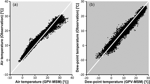
Figure A2. Scatter plot showing predicted (GPV-MSM) and in situ wind speeds observed at the fixed meteorological station (M) (Fig. 1) during the cooling periods in 2017/2018 and 2018/2019.

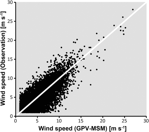
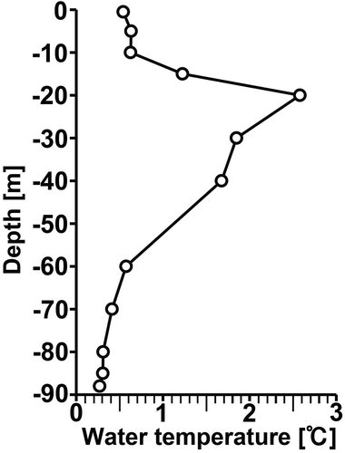
Figure A3. Vertical profiles of the simulated (larger blue dots) and observed water temperatures (red dots) in 2017/2018 at 17B (Fig. 1) during the cooling period from September to March.

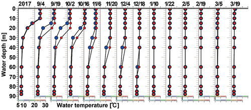
Figure A4. Vertical profiles of the simulated (larger blue dots) and observed water temperatures (red dots) in 2018/2019 at 17B (Fig. 1) during the cooling period from September to March.

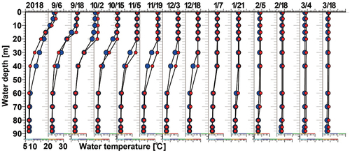
Figure A5. Vertical profiles of RMSE between the simulated and observed water temperature at 17B (Fig. 1) during the cooling period from September to March in 2017/2018 and 2018/2019.