Revisiting the greenhouse effect – a hydrological perspective

Figures & data

Figure 1. Timeline of the observation periods of the eight datasets (not to scale) and atmospheric CO₂ concentration according to Meinshausen et al. (2020). The CO₂ concentration data were downloaded from https://gmd.copernicus.org/articles/13/3571/2020/gmd-13-3571-2020-supplement.zip (accessed 25 August 2023); from the Microsoft Excel file provided at that URL, the data from the column “CO₂ ppm World” of the tabs “T2 – History Year 1750 to 2014” were retrieved.

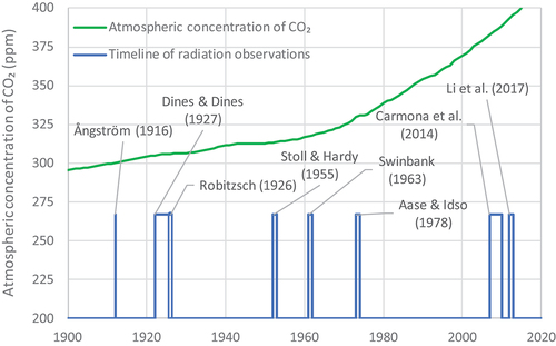
Table 1. Details of the eight datasets used in the study and information about their retrieval.

Dataset no.	Observation year [CO2 concentration], References	Notes
1	1912 [300 ppm] Ångström (1916)	This is probably the earliest record of systematic measurements of $L_{\mathrm{n}}$ (38 in total), conducted by Ångström in Bassour, Algeria, during July–September 1912. The results of all measurements are tabulated in his publication. No preprocessing of the data was necessary except conversion to SI units.
2	1922–1926 [305 ppm] Dines and Dines (1927), Brunt (1932, 1934), Swinbank (1963)	This dataset was the basis of the celebrated Brunt formula, Equation (7)(7) ${\epsilon }_{\mathrm{a}}=0.526+0.065\sqrt{e_{\mathrm{a}}/\mathrm{hPa}}$(7) . The publication by Dines and Dines (1927) contained tables with observations of radiation, including longwave, at Benson, Oxfordshire, UK, during 1922–1926. The tables, which according to Raman (1935) contained 12 monthly mean values, were not found. However, it was possible to make a useful reconstruction of the dataset (ranges rather than individual values), based on the facts that: (a) Brunt (1932, 1934) reports a near perfect correlation with respect to Equation (7), with a correlation coefficient of 0.97; (b) Brunt (1932, 1934) gives the range of $\mathit{e}$ as 7–14 hPa; (c) Swinbank’s (1963) fig. 1 shows that $L_{\mathrm{a}}$ ranged between 237 and 326 $\mathrm{W}{\mathrm{m}}^{-2}$.
3	1926 [306 ppm] Robitzsch (1926), Brunt (1932, 1934), Pekeris (1934)	The original publication by Robitzsch (1926), which contained the measurements, was not found, but his measurements (11 grouped means from 1350 observations taken on 30 clear nights at Lindenberg) were reproduced in tabulated form by Brunt (1932, 1934) and Pekeris (1934). The tabulated data were used here after converting $\mathit{e}$ from mmHg to hPa and recovering from the incorrect value of $\mathit{\sigma }$. Note, though, that Raman (1935) criticized the measurements as possibly influenced by systematic errors.
4	1952–1953 [314 ppm] Stoll and Hardy (1955), Satterlund (1979)	The observations by Stoll and Hardy (1955) were made in Alaska and included some measurements for temperatures below 0°C (down to −55°C). Satterlund (1979, fig. 1), followed by Brutsaert (1991, fig. 6.7), provided these data in graphical form, including in the same convention followed here (see section 4), i.e. $R_{\mathrm{a}}$ calculated by the Brutsaert formula (Equation (4)(4) ${\epsilon }_{\mathrm{a}}=1.24{\left(\frac{{\mathit{e}}_{\mathrm{a}}/\mathrm{hPa}}{T_{\mathrm{a}}/\mathrm{K}}\right)}^{1/7}$(4) ) vs. measured. Satterlund’s figure was digitized, and the units were converted to SI, i.e. from langleys per day ($\mathrm{Ly}{\mathrm{d}}^{-1}=\mathrm{cal}\mathrm{c}{\mathrm{m}}^{-2}{\mathrm{d}}^{-1}$) to $\mathrm{W}{\mathrm{m}}^{-2}$.
5	1961–1962 [318 ppm] Swinbank (1963)	Swinbank (1963) conducted and presented in tabulated form measurements in Australia during 1961–1962, namely Aspendale and Kerang (86 and 5 measurements, respectively), as well as in the Indian Ocean (6 measurements in 1962). The tabulated data were ready for use after the necessary conversion to SI and recovering from the incorrect value of $\mathit{\sigma }$.
6	1973–1974 [330 ppm] Aase and Idso (1978)	Aase and Idso (1978) conducted 65 measurements of longwave radiation at Sidney, Montana, USA (39 for temperatures above 0°C, up to 27°C, and 26 for temperatures below 0°C, down to −30°C). They provided the data in tables, from which they were taken here after conversion from $\mathrm{Ly}{\mathrm{d}}^{-1}$ to $\mathrm{W}{\mathrm{m}}^{-2}$. In addition, Satterlund (1979, fig. 1), followed by Brutsaert (1991, fig. 6.7), provided these data in graphical form, which was cross-checked here and found to agree with the original data.
7	2007–2010 [385 ppm] Carmona et al. (2014)	Carmona et al. (2014) collected data from Tandil in the central-southeastern area of the Buenos Aires province, Argentina, in eight measurement campaigns. The measurements, taken over 840 days, included 3443 hourly observations for clear-sky conditions. As shown in their fig. 2, $L_{\mathrm{a}}$ ranged between 200 and 450 $\mathrm{W}{\mathrm{m}}^{-2}$, $T_{\mathrm{a}}$ between 0 and 36°C, and $\mathit{U}$ between 0.1 and 1. The data are provided in graphical form, including in the same convention followed here (see section 4), i.e. $R_{\mathrm{a}}$ calculated by the Brutsaert formula (Equation (4)(4) ${\epsilon }_{\mathrm{a}}=1.24{\left(\frac{{\mathit{e}}_{\mathrm{a}}/\mathrm{hPa}}{T_{\mathrm{a}}/\mathrm{K}}\right)}^{1/7}$(4) ) vs. measured. The related graph (Carmona et al. 2014, fig. 3d) was digitized and the resulting values, which were originally in SI units, were then ready for processing. It is expected that, because of the large size of the dataset, some of the data points were not identified by the automatic digitization software, but the resulting cloud of points looks identical to that of the original graph.
8	2012–2013 [395 ppm] Li et al. (2017)	Li et al. (2017) processed data from seven Surface Radiation Budget Network (SURFRAD) stations over the contiguous USA covering different climatic conditions and an altitude span from 98 m to 1689 m. Their comprehensive dataset includes 17 127 and 14 052 measurements for clear-sky conditions for 2012 and 2013, respectively. Because of the huge number of data points, their plots illustrate only a random subset to improve the readability of the figures. Therefore, recovery of the data by digitization of their figures was impossible. However, it was possible to make a representative reconstruction of the dataset (ranges rather than individual values), based on the facts that: (a) Li et al. provide a near-perfect recalibration of the Brutsaert formula (Equation (4)(4) ${\epsilon }_{\mathrm{a}}=1.24{\left(\frac{{\mathit{e}}_{\mathrm{a}}/\mathrm{hPa}}{T_{\mathrm{a}}/\mathrm{K}}\right)}^{1/7}$(4) ) on their data, with relative bias of −0.6% and root mean square error (RMSE) of 4.5%; the recalibrated parameters are 1.168 and 1/9, replacing 1.24 and 1/7, respectively; (b) their fig. 2 indicates that $L_a$ ranged between 170 and 450 $\mathrm{W}{\mathrm{m}}^{-2}$; (c) their table 1 provides interquartile ranges for $T_{\mathrm{a}}$, $L_{\mathrm{a}}$ and $\mathit{U}$. Details of the reconstruction method are given in Appendix A.

Figure 2. Plot of downward radiation of the atmosphere L_a calculated by Brutsaert’s formula with its original parameters (Equation (4)(4) ${\epsilon }_{\mathrm{a}}=1.24{\left(\frac{{\mathit{e}}_{\mathrm{a}}/\mathrm{hPa}}{T_{\mathrm{a}}/\mathrm{K}}\right)}^{1/7}$(4) ) vs. measured L_a in all eight datasets. The points correspond to individual measurements, while the lines correspond to reconstructions by envelopes, as described in Table 1 and Appendix A. For the two datasets with the largest number of points (Aase and Idso 1978 and Carmona et al. 2014), the linear regression lines are also shown in the figure, along with their equations.

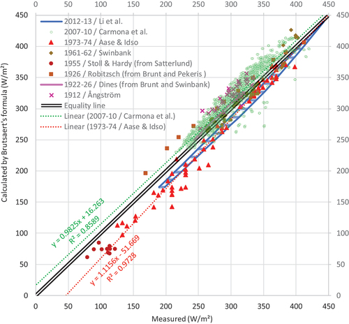
Table A1. Parameters $a^{\prime }$ and $b^{\prime }$ of the generalized Brutsaert formula, ${\epsilon }_{\mathrm{a}}=a^{\prime }{\left({\mathit{e}}_{\mathrm{a}}/T_{\mathrm{a}}\right)}^{\mathit{b}{ }^{\mathrm{\prime }}}$, as recalibrated by Carmona et al. (2014) and Li et al. (2017), and the resulting relative RMSE of the fitting as reported in these publications.

	Original: Brutsaert (1975)	Carmona et al. (2014)	Li et al. (2017)
$a^{\prime }$	1.24	1.11	1.168
$b^{\prime }$	1/7 = 0.143	0.123	1/9 = 0.111
Relative RMSE		4%	4.5%

Figure A1. Cross-check of the reconstruction by envelopes based on the Carmona et al. (2014) dataset, for which both the original points and the envelopes are shown. The reconstruction of Li et al. (2017) is also shown for comparison. The graph is similar to that of Fig. 2, showing the downward radiation of the atmosphere L_a calculated by the Brutsaert formula with its original parameters (Equation (4)(4) ${\epsilon }_{\mathrm{a}}=1.24{\left(\frac{{\mathit{e}}_{\mathrm{a}}/\mathrm{hPa}}{T_{\mathrm{a}}/\mathrm{K}}\right)}^{1/7}$(4) ), vs. measured or reconstructed L_a, but only for the two indicated sets. The points correspond to individual measurements, while the lines correspond to reconstructions by envelopes.

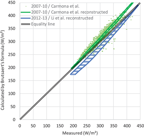
Figure B1. TOA time series of longwave radiation fluxes, as provided by NASA’s CERES, along with linear trend, for (a) all sky and (b) clear sky.

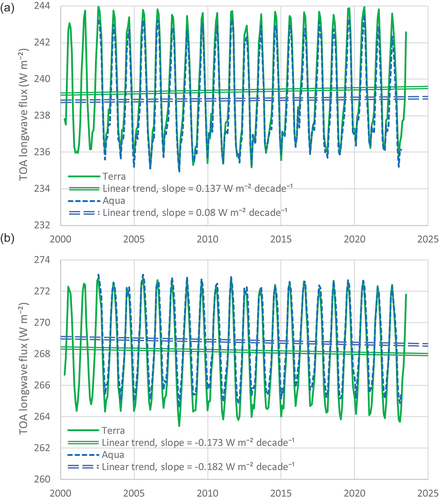
Figure B2. TOA time series of shortwave radiation flux, as provided by NASA’s CERES, along with linear trend, for all sky.

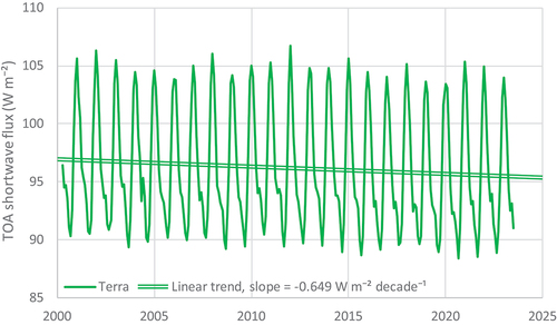
Figure B3. Atmospheric water content (precipitable water), as provided by NASA’s CERES, along with linear trend (which in this case does not exist).

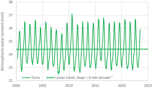
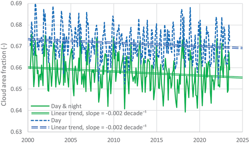
Figure B4. Total cloud area fraction, as provided by NASA’s CERES, along with linear trends.

Meinshausen, M., et al., 2020. The shared socio-economic pathway (SSP) greenhouse gas concentrations and their extensions to 2500. Geoscientific Model Development, 13 (8), 3571–3605. doi:10.5194/gmd-13-3571-2020

 Web of Science ®Google Scholar

Ångström, A., 1916. A study of the radiation of the atmosphere based upon observations of the nocturnal radiation during expeditions to Algeria and to California. Smithsonian Miscellaneous Collections, 65 (3), 159. Available from; https://archive.org/details/smithsonianmisce651916smit/ [ Accessed 25 August 2023].

 Google Scholar

Dines, W.H. and Dines, L.H.G., 1927. Monthly mean values of radiation from various parts of the sky at Benson, Oxfordshire. Memoirs of the Royal Meteorological Society, 2, 11.

 Google Scholar

Brunt, D., 1932. Notes on radiation in the atmosphere. I. Quarterly Journal of the Royal Meteorological Society, 58 (247), 389–420. doi:10.1002/qj.49705824704

 Google Scholar

Brunt, D., 1934. Physical and Dynamical Meteorology. Cambridge, UK: Cambridge University Press, 411. Available from: https://archive.org/details/in.ernet.dli.2015.215092 [ Accessed 25 August 2023].

 Google Scholar

Swinbank, W.C., 1963. Long‐wave radiation from clear skies. Quarterly Journal of the Royal Meteorological Society, 89 (381), 339–348. doi:10.1002/qj.49708938105

 Web of Science ®Google Scholar

Raman, P.K., 1935. Heat radiation from the clear atmosphere at night. Proceedings of the Indian Academy of Sciences – Section A, 1 (11), 815–821. doi:10.1007/BF03035637

 Google Scholar

Robitzsch, M., 1926. Strahlungsstudien. In: H, Hergesell, ed. die Arbeiten des Preußischen Aeronautischen Observatoriums bei Lindenberg. Braunschweig: Verlag Friedrich Vieweg & Sohn, XV, 194–213.

 Google Scholar

Pekeris, C.L., 1934. Note on Brunt’s formula for nocturnal radiation of the atmosphere. Astrophysical Journal, 79, 441–444. doi:10.1086/143552

 Google Scholar

Stoll, A.M. and Hardy, J.D., 1955. Thermal radiation measurements in summer and winter Alaskan climates. Eos, Transactions American Geophysical Union, 36 (2), 213–226.

 Google Scholar

Satterlund, D.R., 1979. An improved equation for estimating long‐wave radiation from the atmosphere. Water Resources Research, 15 (6), 1649–1650. doi:10.1029/WR015i006p01649

 Web of Science ®Google Scholar

Brutsaert, W., 1991. Evaporation into the atmosphere: theory, history and applications. Dordrecht, Netherlands: Springer Science & Business Media, 299.

 Google Scholar

Aase, J.K. and Idso, S.B., 1978. A comparison of two formula types for calculating long‐wave radiation from the atmosphere. Water Resources Research, 14 (4), 623–625. doi:10.1029/WR014i004p00623

 Web of Science ®Google Scholar

Brutsaert, W., 1975. On a derivable formula for long‐wave radiation from clear skies. Water Resources Research, 11 (5), 742–744. doi:10.1029/WR011i005p00742

 Web of Science ®Google Scholar

Carmona, F., Rivas, R., and Caselles, V., 2014. Estimation of daytime downward longwave radiation under clear and cloudy skies conditions over a sub-humid region. Theoretical and Applied Climatology, 115 (1–2), 281–295. doi:10.1007/s00704-013-0891-3

 Web of Science ®Google Scholar

Li, M., Jiang, Y., and Coimbra, C.F., 2017. On the determination of atmospheric longwave irradiance under all-sky conditions. Solar Energy, 144, 40–48. doi:10.1016/j.solener.2017.01.006

 Web of Science ®Google Scholar