A stochastic framework for rainfall intensity–time scale–return period relationships. Part ΙΙ: point modelling and regionalization over Greece

Figures & data

Figure 1. Elevation map of Greece along with the locations of the daily and sub-daily resolution rainfall stations used in the analysis. The coordinate reference system is the GGRS87/Greek Grid (EPSG:2100).

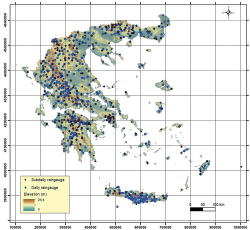
Table 1. Number of stations with data at each time scale.

	Daily raingauges		Sub-daily raingauges
	1 d	2 d	5 min	10 min	15 min	30 min	1 h	2 h	3 h	6 h	12 h	24 h	48 h
Count	503	490	38	128	47	231	273	279	269	280	280	280	223

Table 2. Number of stations with 24-h annual maximum time series longer than 30, 60 and 90 years.

	Length 24 h ≥ 30 years	Length 24 h ≥ 60 years	Length 24 h ≥ 90 years
Sub-daily raingauges	109	2	1
Daily raingauges	383	129	1

Figure 2. Workflow of the regionalization procedure. Yellow boxes correspond to procedures for simultaneous parameter estimation (shared parameters), green ones correspond to the final regionalization procedures and the remaining white boxes denote procedures that are intermediate and auxiliary to the regionalization.

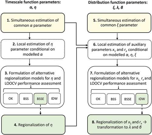
Figure 3. Regionalized η parameter resulting from the application of the BSSE model. The coordinate reference system is the GGRS87/Greek Grid (EPSG:2100).

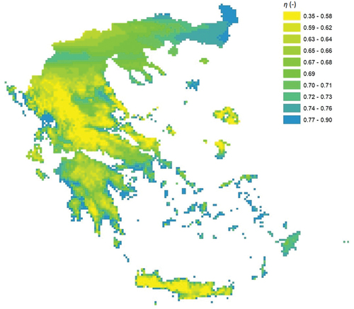
Table 3. Entire dataset statistics for η, x₁ and $r_x$.

Interpolation method	MBE	MAE	RMSE	R^2	EF
η
BSS	0.00	0.07	0.08	0.25	0.26
BSSE*	0.00	0.05	0.06	0.57	0.57
OK	0.00	0.03	0.03	0.91	0.88
IDW	0.00	0.01	0.02	0.98	0.98
x1
BSS	0.00	0.02	0.04	0.28	0.27
BSSE	0.00	0.38	0.54	0.63	0.43
OK	0.00	0.21	0.31	0.90	0.88
IDW*	0.01	0.13	0.24	0.93	0.92
$r_x$
BSS	0.00	0.17	0.26	0.26	0.20
BSSE	0.00	0.18	0.26	0.27	0.26
OK	0.00	0.15	0.23	0.38	0.33
IDW*	0.01	0.13	0.24	0.93	0.92

*denotes best performance according to LOOCV.

Table 4. Leave-one-out cross-validation statistics for η, x₁ and $r_x$.

Interpolation method	MBE	MAE	RMSE	R^2	EF
η
BSS	0.00	0.07	0.08	0.28	0.28
BSSE*	0.00	0.06	0.07	0.40	0.40
OK	0.00	0.07	0.08	0.30	0.28
IDW	0.00	0.06	0.08	0.28	0.28
x1
BSS	0.00	0.02	0.04	0.18	0.17
BSSE	–0.01	0.51	0.75	0.43	0.40
OK	0.00	0.43	0.64	0.49	0.47
IDW*	0.01	0.44	0.65	0.49	0.48
$r_x$
BSS	0.00	0.18	0.27	0.16	0.12
BSSE	0.00	0.18	0.27	0.18	0.15
OK	0.00	0.18	0.28	0.08	0.07
IDW*	–0.01	0.17	0.29	0.32	0.28

*denotes best performance according to LOOCV.

Figure 4. Theoretical (Pareto) and empirical distribution of the standardized daily rainfall depth for the case where dependence bias is considered ($\mathrm{\Theta }$ = −0.04) and the case where dependence is neglected ($\mathrm{\Theta }$ = 0).

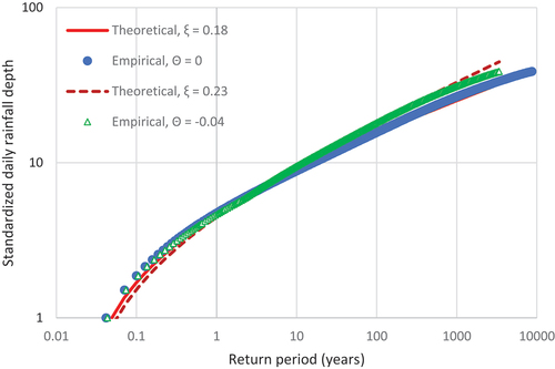
Figure 5. Probability distribution of simulated tail index ξ_e, generated from a Pareto distribution with scale parameter λ = 1 and theoretical tail index ξ = 0.01 and ξ = 0.18 assuming that the generated values are the upper 2% of a larger sample. The results are obtained from 70 simulated series of 70 values, for each of which the empirical values λ_e and ξ_e are estimated by optimization. In addition to the empirical distributions, the theoretical normal distributions N(ξ – ζ, σ) are also shown, where ζ = −0.03 is the bias and σ the standard deviation, with values as in the legend of the figure, both estimated with Monte Carlo.

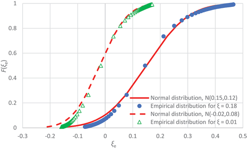
Figure 6. Probability distribution of simulated standardized daily rainfall, generated from a Pareto distribution with scale parameter λ = 1 and tail index ξ = 0.18 assuming that the simulated values are the upper 2% of a larger sample. In addition to the median and 90% confidence limits of the simulated empirical distributions, two individual simulated distributions are shown with an empirical (optimized) index ξ_e approximately equal to its upper and lower confidence limits (where the high and low ξ_e are 0.35 and −0.02, respectively).

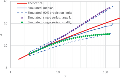
Figure 7. Regionalized β (years) and λ (mm/h) parameters using the IDW method. The coordinate reference system is the GGRS87/Greek Grid (EPSG:2100).

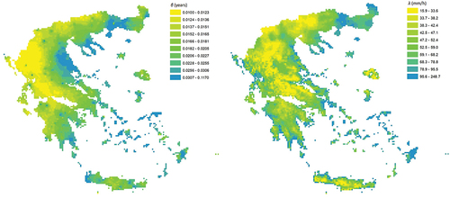
Figure 8. Dimensionless (%) mean deviation of the model from the empirical K-moments (a) and dimensionless (%) RMSE (b), both averaged over all time scales available from the daily and sub-daily raingauges. Set A indicates the sub-daily raingauges used for the full calibration of the ombrian relationships, while Set B denotes the sub-daily raingauges used only for the calibration of the parameters of the time scale function.

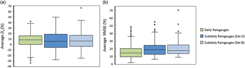
Figure 9. Dimensionless (%) deviation of the regional model from the local model (estimated from the set of sub-daily raingauges) for 1 h scale (a) and 24 h scale (b) and different return periods.

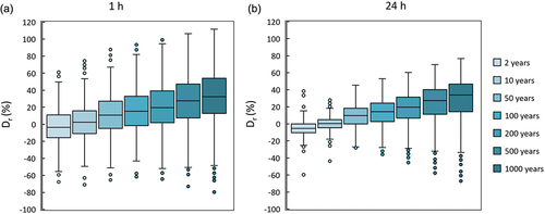
Figure 10. Theoretical and empirical distributions of annual maximum intensities at scales of 5 min to 48 h (depending on the available samples) from the sub-daily stations of Limnos (a) and Lofos Nymphon-Athens (b). For the latter, the empirical intensities at the 24 h and 48 h scales from the daily raingauge are shown as well. The empirical intensities plotted based on order statistics are also shown for validation.

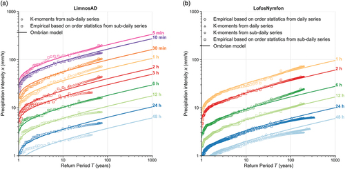
Figure 11. Left panel: estimated rainfall depth (mm) for 1 h and return periods 50, 100 and 1000 years, right panel: estimated rainfall depth (mm) for 24 h and return periods 50, 100 and 1000 years. Quantile classification is employed for all legends. The coordinate reference system is the GGRS87/Greek Grid (EPSG:2100).

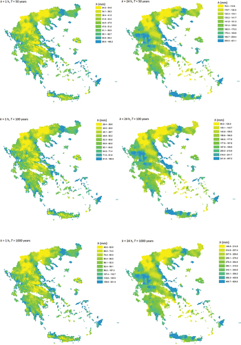
Figure A1. Estimate of parameter $\mathit{\alpha }$ vs temporal resolution of the rain recorder.

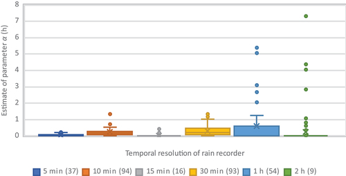
Figure A2. Average of estimated $\mathit{\alpha }$ parameters vs the temporal resolution of the rain recorders.

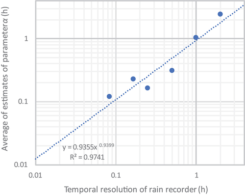
Figure A3. Geographic distribution of the independently estimated ξ parameters.

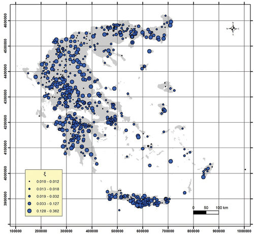
Figure B1. Dimensionless (%) mean deviation of the model from the empirical K-moments (a) and dimensionless (%) root mean square error (RMSE, (b)), for all time scales available from the daily raingauges.

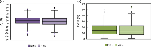
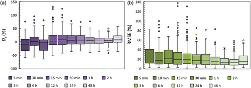
Figure B2. Dimensionless (%) mean deviation of the model from the empirical K-moments (a) and dimensionless (%) RMSE (b), for all time scales available from the sub-daily raingauges.

Data availability statement

The data of the General Directorate of Water of the Greek Ministry of Environment and Energy are available online for free from the Hydroscope platform (http://www.hydroscope.gr/, accessed 25 March 2023). All other data belong to other Greek organizations and are not publicly available.