The effects of simulated vision impairment on performance in football

Figures & data

Table 1. Current classes based on visual acuity and visual field; LogMAR 1.0 represents the current MIC (World Health Organisation, 2004.).

Class	Visual acuity (LogMAR)	Visual field (diameter)	Description
B3	1.0 to 1.4	Less than 40 degrees	Limited visual acuity and/or visual field in both eyes.
B2	1.5 to 2.6	Less than 10 degrees	Severely limited visual acuity and/or visual field in both eyes.
B1	Poorer than 2.6	Cannot be B1 with only loss of visual field	A player can typically distinguish only light from dark or is not able to perceive light.

Table 2. Mean ± SD (min – max) for each level of simulated impairment in this study.

Level	How Simulated	Visual Acuity LogMAR (ETDRS)	Contrast Sensitivity LogCS (MARS)
Control	No simulation	−0.14±0.09 (−0.30–0.06)	1.85±0.05 (1.76–1.92)
Clear Lens	Stock clear lens	−0.14±0.14 (−0.40–0.26)	1.85±0.06 (1.68–1.92)
Level 1	Four layers of 258	0.51±.018 (0.16–0.84)	1.03±0.17 (0.48–1.36)
Level 2	Five layers of 258	0.83±0.11 (0.56–0.98)	0.77±0.19 (0.08–1.00)
Level 3	Six layers of 258	1.09±0.23 (0.70–1.60)	0.49±0.17 (0.20–0.84)
Level 4	Seven layers of 258	1.21±0.23 (0.88–1.60)	0.25±0.13 (0.00–0.44)
Level 5	One layer of 256	1.50±0.11 (1.30–1.64)	0.15±0.19 (0.00–0.52)
Level 6	One layer of 253	1.84±0.18 (1.60–2.50)	0.03±0.09 (0.00–0.40)

ETDRS = Early Treatment Diabetic Retinopathy Study Chart. MARS = Mars Perceptrix Contrast Sensitivity Test.

Figure 1. Schematic showing the set-up and execution of the vision impaired football skills test (Runswick et al., 2022).

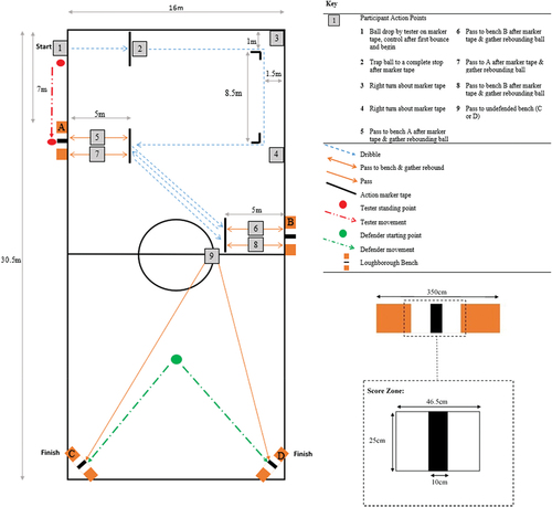
Figure 2. The level of impairment experienced across each simulation (levels 1–6, control and clear) for visual acuity (LogMAR) and contrast sensitivity (LogCS). Plots show either MARS chart (a) or app (b) used to measure contrast sensitivity.

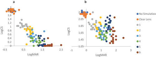
Figure 3. Mean (diamond) and individual (small circle) percentages of habitual technical performance at each level of impairment (1–6) for visual acuity (a), contrast sensitivity measured using a MARS chart (b) and contrast sensitivity measured using the app (c). The solid lines show habitual performance, the dotted lines show the boundaries of expected performance.

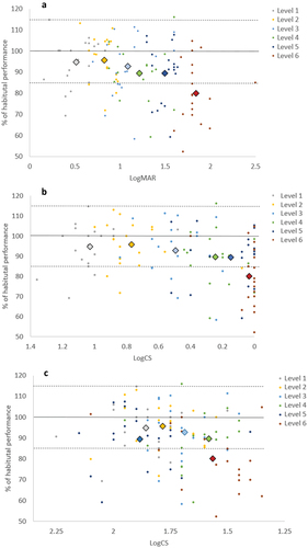
Figure 4. Mean (diamond) and individual (small circle) percentages of habitual anticipation performance at each level of impairment (1–6) for visual acuity (a), contrast sensitivity measured using a MARS chart (b) and contrast sensitivity measured using the app (c). The solid lines show habitual performance, the dotted lines show the boundaries of expected performance.

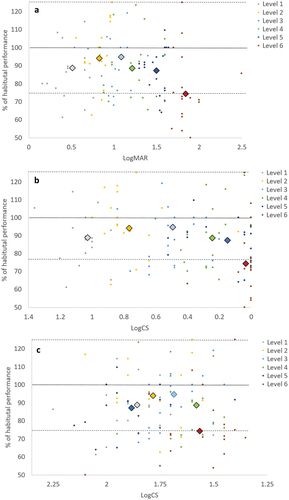
Figure 5. The sensitivity and specificity for different possible MICs for visual acuity for technical (a) and anticipation performance (c) and contrast sensitivity for technical (b) and anticipation performance (d).

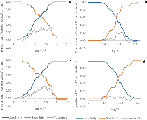
Figure 6. Unconstrained decision tree model for technical performance (a) the full decision tree prior to pruning. (b) the pruned decision tree. In this case, the optimum number of nodes was equal to the original five.

Figure 7. Unconstrained decision tree model for anticipation performance. (a) the full decision tree prior to pruning. (b) the pruned decision tree.

World Health Organisation. (2004). International statistical classification of disease and related Health problems. https://www.who.int/standards/classifications/classification-of-diseases

 Google Scholar

Runswick, O. R., Rawlinson, A., Datson, N., & Allen, P. M. (2022). A valid and reliable test of technical skill in vision impaired football. Science and Medicine in Football, 6(1), 89–97. https://doi.org/10.1080/24733938.2021.1885725

 PubMedGoogle Scholar

Data availability statement

Data associated with this submission is available at: https://osf.io/7udzq/?view_only=72cd96a4b30f4f05b02b9d2f89f2053f